
Abstract. In my research, I study the electrical automation control of the mobile behavior of an industrial robot. I treat the motion of an industrial robot as a multivariable coupled dynamic optimization problem. When an industrial robot moves through a production environment, different devices often use different communication interface standards, and this inconsistency makes accurate data transmission difficult. As a result, the integrated industrial robot can show low control precision during motion, task switching, and trajectory tracking. To address this problem, I propose an electrical automation control method for the mobile behavior of an industrial robot. I first obtain the pose of the industrial robot at the current time and construct a mathematical model of the industrial robot. When the industrial robot moves, I set the motor speed of the industrial robot and use electrical automation technology for connection and integrated control. In my experiments, the actual rotational speed of the industrial robot motor closely matches the expected rotational speed and remains stable at approximately \(2500\ \text{r/min}\). My method guides the industrial robot through an environment with obstacles and produces a feasible movement path. The lowest fluctuation rate of the mobile behavior is \(0.5\%\), the minimum trajectory deviation is \(0.12\ \text{mm}\), the shortest task switching time is \(20\ \text{ms}\), and the highest task execution efficiency is \(95\%\). These results satisfy the control precision requirements of industrial production. The key terms of my study include industrial robot, electrical automation technology, electrical integration, device control, electrical automation, and differentiated demand.
Introduction. In my view, the transformation and upgrading of manufacturing and the growth of intelligent manufacturing have made the industrial robot a central piece of equipment in the modern industrial system. The precision, flexibility, and intelligence of the mobile behavior of an industrial robot directly affect the efficiency and quality of a production line. Traditional industrial robot systems often depend on fixed trajectory planning and open-loop control. In complex dynamic environments, unstructured scenes, and human-robot collaboration tasks, such industrial robot systems can show insufficient adaptability, delayed response, and high energy consumption. These limitations are key bottlenecks that restrict the application of the industrial robot in high-end manufacturing. I observe three major trends in the electrical automation control of the mobile behavior of an industrial robot. The first trend is multi-sensor fusion perception. The second trend is intelligent algorithm-driven decision making. The third trend is networked collaborative control. Electrical automation technology integrates sensors, drivers, controllers, and communication networks. Through this integration, electrical automation technology can realize closed-loop control of the movement, perception, and decision-making processes of an industrial robot.
Some existing methods have tried to improve the trajectory tracking of mobile robots. One approach constructs kinematic and dynamic models and applies an improved linear active disturbance rejection control strategy. That approach designs a backstepping control policy, sets target speed parameters, and uses a linear extended state observer. It also modifies a conventional control law with an improved sigmoid function so that the actual speed of the robot approaches the preset speed. Such a method can improve trajectory tracking accuracy, dynamic response, and disturbance rejection in simulation. However, when a dynamic obstacle appears or a task changes, the robot may need to pause and replan, which reduces efficiency. Another approach uses an improved nonlinear sliding mode control for wheeled robot trajectory control. It builds a trajectory tracking error model, designs a power-exponential time-varying sliding surface, avoids singular states by adjusting sliding surface parameters, and proves stability with a Lyapunov function. It designs a composite control law for linear velocity and angular velocity. The tracking error converges to zero in finite time, and the method shows strong convergence, tracking accuracy, and robustness. However, this method depends on a single sensor feedback channel and lacks multimodal information fusion. Another approach uses configuration software to control an industrial robot. It builds a dynamic model based on kinematics theory, solves motion parameters in Cartesian space, and adds trajectory tracking capability. This approach can increase the compliance of the motion of an industrial robot, but communication between the configuration software and the robot controller may be unstable. When communication is unstable, motion control commands may not be transmitted accurately, and the motion precision of the industrial robot can degrade.
In practical applications, these methods are often unable to achieve precise control of the motion process of an industrial robot. They may not satisfy the current requirements of industrial production and industrial robot applications. To reduce this gap, I propose an electrical automation control method for the mobile behavior of an industrial robot. My method combines pose estimation, mathematical modeling, motor speed setting, and electrical automation integration. I focus on the industrial robot as an integrated electromechanical system. I use the term industrial robot repeatedly because the behavior of the industrial robot is the central object of my control design. I also consider the industrial robot communication interface, the industrial robot motor drive, the industrial robot controller, and the industrial robot task execution process as parts of one electrical automation architecture.
Problem Formulation. I formulate the mobile behavior control of an industrial robot as a multivariable coupled dynamic optimization problem. The state of the industrial robot includes position, orientation, joint variables, motor speeds, and communication states. The control input includes motor voltage, current, pulse width modulation duty cycle, and high-level velocity commands. The output includes the actual pose, actual speed, trajectory error, and task completion status. In a typical industrial robot cell, multiple devices exchange data. These devices may include programmable logic controllers, servo drives, sensors, vision systems, safety modules, and human-machine interfaces. If the communication interface standards of these devices are not unified, the industrial robot may receive delayed, incomplete, or inconsistent data. Therefore, I define the control problem as a coupled optimization problem with communication constraints.
I define the generalized state vector of the industrial robot as follows:
$$
\mathbf{x}(t) =
\begin{bmatrix}
x(t) & y(t) & z(t) & \theta(t) & \dot{x}(t) & \dot{y}(t) & \dot{\theta}(t)
\end{bmatrix}^{T}
$$
I define the control input vector of the industrial robot as follows:
$$
\mathbf{u}(t) =
\begin{bmatrix}
v_l(t) & v_r(t) & a_l(t) & a_r(t)
\end{bmatrix}^{T}
$$
Here, \(v_l(t)\) and \(v_r(t)\) are the left and right motor speed commands of the industrial robot, and \(a_l(t)\) and \(a_r(t)\) are the corresponding acceleration commands. I define the output vector of the industrial robot as follows:
$$
\mathbf{y}(t) =
\begin{bmatrix}
x(t) & y(t) & \theta(t) & \omega(t)
\end{bmatrix}^{T}
$$
The general state-space form of the industrial robot mobile behavior is:
$$
\dot{\mathbf{x}}(t) = \mathbf{f}(\mathbf{x}(t), \mathbf{u}(t), \mathbf{d}(t), t)
$$
$$
\mathbf{y}(t) = \mathbf{h}(\mathbf{x}(t), \mathbf{u}(t), t)
$$
where \(\mathbf{d}(t)\) represents disturbances from load changes, surface friction, sensor noise, communication delay, and obstacle-induced path adjustments. My goal is to design an electrical automation controller for the industrial robot so that the actual output \(\mathbf{y}(t)\) tracks the desired output \(\mathbf{y}_d(t)\) with bounded error. The desired output is generated by a trajectory planner and a task manager. The electrical automation controller must also maintain stability when the communication quality changes or when the load of the industrial robot changes.
Pose Acquisition and Mathematical Modeling. The mathematical modeling of the mobile behavior of an industrial robot is essentially an abstraction of kinematics, dynamics, and environmental interaction. I use the model to create solvable equations for control. Kinematics modeling focuses on the mapping between the position and posture of the end effector of the industrial robot in task space and the joint space variables. I obtain the pose of the industrial robot at the current time by using the following discrete update equations:
$$
\begin{cases}
x(t) = x(t-1) + \sigma_x \\
y(t) = y(t-1) + \sigma_y \\
z(t) = z(t-1) + \sigma_z
\end{cases}
$$
In these equations, \(x(t)\), \(y(t)\), and \(z(t)\) represent the posture of the mobile behavior of the industrial robot. The terms \(\sigma_x\), \(\sigma_y\), and \(\sigma_z\) represent disturbance components along the \(x\), \(y\), and \(z\) axes. These disturbance components can come from encoder quantization, wheel slip, uneven ground, or communication jitter. I use the pose information to determine the real-time pose of the industrial robot. I then treat this real-time pose as the input for the next stage of motion control.
I also define a pose error transformation for the industrial robot. The transformation aligns the current pose of the industrial robot with the desired movement direction. I use the following expression:
$$
P_e =
\begin{bmatrix}
\cos\theta_d & \sin\theta_d & 0 \\
-\sin\theta_d & \cos\theta_d & 0 \\
0 & 0 & 1
\end{bmatrix}
\begin{bmatrix}
e_x \\
e_y \\
e_\phi
\end{bmatrix}
$$
In this equation, \(\theta_d\) is the angle between the movement direction and the motion direction of the industrial robot. The terms \(e_x\), \(e_y\), and \(e_\phi\) are the differences between the target position and the starting position, including the orientation error. The transformed error \(P_e\) allows the electrical automation controller to evaluate the deviation of the industrial robot from the planned path in a local coordinate frame. This local evaluation is important because the industrial robot may need to rotate, translate, and adjust its speed simultaneously while avoiding obstacles.
I summarize the main symbols used in my model in the following table.
| Symbol | Meaning | Role in Industrial Robot Control |
|---|---|---|
| \(x(t), y(t), z(t)\) | Pose components of the industrial robot | Describe the current location of the industrial robot |
| \(\theta_d\) | Desired movement angle | Aligns the industrial robot with the target direction |
| \(\sigma_x, \sigma_y, \sigma_z\) | Disturbance components | Represent uncertainty in the motion of the industrial robot |
| \(e_x, e_y, e_\phi\) | Pose errors | Measure tracking deviation of the industrial robot |
| \(v_l, v_r\) | Left and right motor speeds | Control the differential drive of the industrial robot |
| \(T\) | Sampling period | Defines the discrete control interval for the industrial robot |
| \(\Delta_l, \Delta_r\) | Left and right wheel travel distances | Estimate the movement of the industrial robot |
| \(P_e\) | Transformed pose error | Provides local error coordinates for the industrial robot |
Kinematic Model of the Industrial Robot. I model the industrial robot as a differential-drive mobile platform for the purpose of mobile behavior control. The kinematic model relates the linear velocity and angular velocity of the industrial robot to its pose derivatives. I define the linear velocity \(v(t)\) and angular velocity \(\omega(t)\) of the industrial robot as follows:
$$
v(t) = \frac{v_r(t) + v_l(t)}{2}
$$
$$
\omega(t) = \frac{v_r(t) – v_l(t)}{L}
$$
where \(L\) is the distance between the left and right wheels of the industrial robot. The pose evolution of the industrial robot is:
$$
\begin{bmatrix}
\dot{x}(t) \\
\dot{y}(t) \\
\dot{\theta}(t)
\end{bmatrix}
=
\begin{bmatrix}
\cos\theta(t) & 0 \\
\sin\theta(t) & 0 \\
0 & 1
\end{bmatrix}
\begin{bmatrix}
v(t) \\
\omega(t)
\end{bmatrix}
$$
By substituting the wheel speed definitions into the kinematic model, I obtain a direct relationship between the motor speed commands and the pose of the industrial robot:
$$
\begin{bmatrix}
\dot{x}(t) \\
\dot{y}(t) \\
\dot{\theta}(t)
\end{bmatrix}
=
\begin{bmatrix}
\frac{\cos\theta(t)}{2} & \frac{\cos\theta(t)}{2} \\
\frac{\sin\theta(t)}{2} & \frac{\sin\theta(t)}{2} \\
-\frac{1}{L} & \frac{1}{L}
\end{bmatrix}
\begin{bmatrix}
v_l(t) \\
v_r(t)
\end{bmatrix}
$$
This equation shows that the mobile behavior of the industrial robot is coupled. A change in the left motor speed or the right motor speed affects both translation and rotation. Therefore, I cannot treat the motor speed control of the industrial robot as independent single-loop control. I need an integrated electrical automation control method that coordinates the left and right drives of the industrial robot.
Dynamic Model and Load Disturbance. For the dynamic behavior of the industrial robot, I use a simplified model that includes inertia, viscous friction, motor torque, and load disturbance. I define the dynamic equation of the industrial robot as:
$$
M(q)\ddot{q} + C(q,\dot{q})\dot{q} + G(q) + F(\dot{q}) = \tau + \tau_d
$$
In this equation, \(q\) is the generalized coordinate vector of the industrial robot, \(M(q)\) is the inertia matrix, \(C(q,\dot{q})\) is the Coriolis and centrifugal term, \(G(q)\) is the gravity term, \(F(\dot{q})\) is the friction term, \(\tau\) is the control torque, and \(\tau_d\) is the disturbance torque. For a mobile industrial robot on a flat floor, I can reduce the model to a wheel-level dynamic equation:
$$
J_w \dot{\omega}_l + B_w \omega_l = \tau_l – r F_l
$$
$$
J_w \dot{\omega}_r + B_w \omega_r = \tau_r – r F_r
$$
Here, \(J_w\) is the wheel inertia, \(B_w\) is the viscous damping coefficient, \(r\) is the wheel radius, \(\omega_l\) and \(\omega_r\) are the wheel angular speeds, \(\tau_l\) and \(\tau_r\) are the motor torques, and \(F_l\) and \(F_r\) are the ground reaction forces. The electrical automation controller must compensate for changes in \(F_l\) and \(F_r\) when the industrial robot carries different payloads or moves over different surfaces.
I define the tracking error of the industrial robot as:
$$
e(t) = q_d(t) – q(t)
$$
where \(q_d(t)\) is the desired trajectory of the industrial robot and \(q(t)\) is the actual trajectory. I use a proportional-integral-derivative control structure in the electrical automation layer:
$$
u(t) = K_p e(t) + K_i \int_0^t e(\tau) d\tau + K_d \frac{de(t)}{dt}
$$
The gains \(K_p\), \(K_i\), and \(K_d\) are tuned according to the load and communication conditions of the industrial robot. I use the derivative term to improve damping, the integral term to reduce steady-state error, and the proportional term to increase response speed. This control structure is implemented in the programmable logic controller and the servo drive network of the industrial robot.
Motor Speed Setting for the Industrial Robot. When the industrial robot moves, I set the motor speed of the industrial robot. I use \(v_l\) and \(v_r\) to denote the predicted movement speeds of the left wheel and the right wheel of the industrial robot motor. When the industrial robot moves along a straight line, the movement angle is zero. I use \(V_l\) and \(V_r\) to denote the actual movement speeds of the left and right wheels. I estimate the predicted speeds from the wheel travel distance and the sampling period:
$$
v_l = \frac{\Delta_l \times v_l}{T}
$$
$$
v_r = \frac{\Delta_r \times v_r}{T}
$$
To avoid ambiguity in the notation, I also define the wheel angular speed form used by the servo drive of the industrial robot:
$$
v_l^{cmd} = r \omega_l^{cmd}
$$
$$
v_r^{cmd} = r \omega_r^{cmd}
$$
where \(\omega_l^{cmd}\) and \(\omega_r^{cmd}\) are the commanded angular speeds of the left and right motors of the industrial robot. The actual speeds are measured by encoders:
$$
v_l^{act} = r \omega_l^{act}
$$
$$
v_r^{act} = r \omega_r^{act}
$$
The speed error of the industrial robot is:
$$
e_v(t) =
\begin{bmatrix}
v_l^{cmd}(t) – v_l^{act}(t) \\
v_r^{cmd}(t) – v_r^{act}(t)
\end{bmatrix}
$$
I use this error to adjust the motor drive output. The electrical automation controller updates the drive command at each sampling period \(T\). The update law is:
$$
v_l^{cmd}(k+1) = v_l^{cmd}(k) + K_{v,l} e_{v,l}(k)
$$
$$
v_r^{cmd}(k+1) = v_r^{cmd}(k) + K_{v,r} e_{v,r}(k)
$$
The speed control of the industrial robot is therefore not only a motor-level task but also a system-level task. The speed commands must be consistent with the planned path, the obstacle avoidance behavior, and the task priority of the industrial robot. I list the main speed control variables in the following table.
| Variable | Description | Control Meaning for the Industrial Robot |
|---|---|---|
| \(v_l^{cmd}\) | Commanded left wheel speed | Sets the left movement of the industrial robot |
| \(v_r^{cmd}\) | Commanded right wheel speed | Sets the right movement of the industrial robot |
| \(v_l^{act}\) | Actual left wheel speed | Measures left drive response of the industrial robot |
| \(v_r^{act}\) | Actual right wheel speed | Measures right drive response of the industrial robot |
| \(e_{v,l}\) | Left speed error | Drives left motor correction of the industrial robot |
| \(e_{v,r}\) | Right speed error | Drives right motor correction of the industrial robot |
| \(K_{v,l}\) | Left speed gain | Tunes left speed convergence of the industrial robot |
| \(K_{v,r}\) | Right speed gain | Tunes right speed convergence of the industrial robot |
Electrical Automation Control Architecture. Based on the motion control requirements of the industrial robot, I design a programmable logic controller program with five modules. These modules are the power-on initialization module, the communication normality judgment module, the positioning module, the origin return module, and the alarm module. I use electrical automation technology to connect these modules. The electrical automation architecture of the industrial robot provides integrated logic control. I use a terminal block to connect the programmable logic controller modules. I also connect a computer to monitor the communication signals of the industrial robot. In this way, I achieve integrated control of the units of the industrial robot.
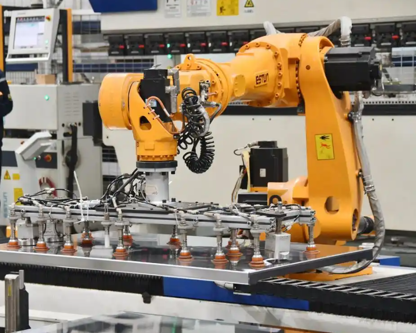
In the logic control integration, electrical automation technology uses advanced automation control logic to achieve precise control of the motion process of the industrial robot. The programmable logic controller program acts as the control core. Through the terminal block, the programmable logic controller connects the modules and realizes electrical automation control of the mobile behavior of the industrial robot. The control architecture includes a sensing layer, a control layer, a communication layer, and an execution layer. The sensing layer collects encoder data, proximity sensor data, vision data, and safety signals. The control layer runs the trajectory planner, the speed controller, and the task scheduler. The communication layer uses industrial protocols and interface conversion to connect the industrial robot with other devices. The execution layer includes servo drives, motors, brakes, and end effectors.
I summarize the programmable logic controller modules for the industrial robot in the following table.
| Module | Function | Relation to the Industrial Robot |
|---|---|---|
| Power-on initialization | Sets parameters, resets registers, checks drives | Prepares the industrial robot for motion |
| Communication normality judgment | Checks data links and interface standards | Ensures reliable data exchange for the industrial robot |
| Positioning | Processes pose and trajectory targets | Guides the industrial robot to the required pose |
| Origin return | Restores reference position and encoder zero | Maintains repeatability of the industrial robot |
| Alarm | Detects faults, overloads, and communication errors | Protects the industrial robot and the production line |
Communication and Electrical Integration. The communication interface standard is a critical issue for the industrial robot. When different devices use different standards, the industrial robot controller may receive data in different formats, at different rates, and with different time stamps. I use an electrical automation integration layer to normalize these data. The integration layer performs protocol conversion, data validation, time synchronization, and priority scheduling. I define the communication cycle of the industrial robot as:
$$
T_{comm} = T_{frame} + T_{queue} + T_{decode} + T_{ack}
$$
where \(T_{frame}\) is the frame transmission time, \(T_{queue}\) is the queuing delay, \(T_{decode}\) is the decoding time, and \(T_{ack}\) is the acknowledgment time. The total control cycle of the industrial robot is:
$$
T_{scan} = T_{in} + T_{logic} + T_{out} + T_{comm}
$$
I require \(T_{scan}\) to be smaller than the maximum allowable control period of the industrial robot. If \(T_{scan}\) exceeds the limit, the industrial robot may show lag, overshoot, or instability. Therefore, I assign higher priority to safety messages, encoder feedback, and motor speed commands. I assign lower priority to non-critical logging and human-machine interface updates. This priority scheduling improves the real-time performance of the industrial robot without increasing the hardware cost significantly.
I also define a communication reliability index for the industrial robot:
$$
R_{comm} = \frac{N_{valid}}{N_{total}} \times 100\%
$$
where \(N_{valid}\) is the number of valid communication frames and \(N_{total}\) is the total number of frames. In my design, \(R_{comm}\) must remain above a threshold \(R_{min}\). If \(R_{comm} < R_{min}\), the alarm module of the industrial robot triggers a safe state. The safe state may include speed reduction, path holding, or emergency stop, depending on the task and the environment.
Trajectory Planning and Obstacle Avoidance. I plan the trajectory of the industrial robot in the task space. The trajectory planner generates a sequence of poses and velocities. The obstacle avoidance module modifies the trajectory when an obstacle is detected. I define the obstacle avoidance cost function as:
$$
J = \sum_{k=0}^{N} \left( \|x_k – x_{goal}\|_Q^2 + \|u_k\|_R^2 + \rho \sum_{j=1}^{M} \frac{1}{\|x_k – o_j\|^2 + \epsilon} \right)
$$
In this equation, \(x_k\) is the state of the industrial robot at step \(k\), \(x_{goal}\) is the goal state, \(u_k\) is the control input, \(o_j\) is the position of obstacle \(j\), \(Q\) and \(R\) are weight matrices, \(\rho\) is the obstacle penalty weight, and \(\epsilon\) is a small positive constant. The cost function penalizes distance to the goal, control effort, and proximity to obstacles. By minimizing this cost function, the industrial robot can generate a feasible path that avoids obstacles and reaches the target.
I use a receding-horizon strategy. At each control step, I solve a finite-horizon optimization problem for the industrial robot. I apply only the first control input to the industrial robot. Then I update the state and repeat the optimization. This strategy allows the industrial robot to respond to dynamic changes. If a new obstacle appears, the industrial robot can replan without a long pause. The task switching time is therefore reduced.
I define the trajectory deviation of the industrial robot as:
$$
d_{traj}(t) = \sqrt{(x(t)-x_d(t))^2 + (y(t)-y_d(t))^2}
$$
I define the fluctuation rate of the mobile behavior of the industrial robot as:
$$
F_{rate} = \frac{\max(d_{traj}) – \min(d_{traj})}{\text{mean}(d_{traj})} \times 100\%
$$
These metrics allow me to evaluate the precision and stability of the industrial robot. I use them in the experimental analysis.
Experimental Setup. To validate the effectiveness of my electrical automation control method for the mobile behavior of an industrial robot, I select an actual production line of a large manufacturing enterprise as the experimental scenario. I use a six-degree-of-freedom industrial robot as the experimental object. The industrial robot has a working radius of \(1900\ \text{mm}\) and a repeat positioning accuracy of \(\pm 0.05\ \text{mm}\). These specifications meet the requirements of high-precision industrial production. In the experiment, I do not rely only on conventional control command tests. I also introduce dynamic path planning tests in complex environments. These tests evaluate the motion control precision and stability of the industrial robot under different working conditions.
I list the main technical parameters of the industrial robot in the following table.
| Parameter | Value | Importance for the Industrial Robot |
|---|---|---|
| Working radius | \(1900\ \text{mm}\) | Defines the reachable workspace of the industrial robot |
| Repeat positioning accuracy | \(\pm 0.05\ \text{mm}\) | Supports high-precision tasks of the industrial robot |
| Typical power consumption | \(350\ \text{W}\) | Indicates energy demand of the industrial robot |
| Tool communication | RS485 | Connects the tool interface of the industrial robot |
| Base joint motion range | \(\pm 360^\circ\) | Provides rotational freedom of the industrial robot |
| Base joint maximum speed | \(120^\circ/\text{s}\) | Limits fast base motion of the industrial robot |
| Standard cruise rate | \(0.3\ \text{m/s}\) | Sets normal mobile speed of the industrial robot |
| Operating temperature range | \(0^\circ\text{C}\) to \(60^\circ\text{C}\) | Defines environmental tolerance of the industrial robot |
| Spindle rated speed | \(2500\ \text{r/min}\) | Establishes the main speed reference of the industrial robot |
| Rapid movement capability | \(0.6\ \text{m/s}\) | Supports fast repositioning of the industrial robot |
| Wrist joint motion range | \(\pm 360^\circ\) | Provides wrist orientation of the industrial robot |
| Wrist joint maximum speed | \(260^\circ/\text{s}\) | Limits wrist rotation speed of the industrial robot |
Speed Tracking Results. I use my method to control the mobile behavior of the industrial robot. The motor speed control result of the industrial robot is a key indicator. In the initial stage, the actual speed of the industrial robot is lower than the expected speed. However, the actual speed rises quickly and approaches the expected speed within about \(20\ \text{s}\). After that, the actual speed fluctuates in a small range around the expected speed. The actual speed and the expected speed are nearly coincident and remain stable at approximately \(2500\ \text{r/min}\). This result indicates that my control method can make the motor of the industrial robot run at the expected speed. The control system has good stability and can maintain speed stability in a short time. This behavior satisfies the requirements of the mobile behavior of the industrial robot. The fast response and short adjustment time also show that the control system has good dynamic performance. It can respond to speed changes in time and adapt to different working conditions.
I quantify the speed tracking performance of the industrial robot in the following table.
| Metric | Observed Value | Interpretation for the Industrial Robot |
|---|---|---|
| Expected speed | \(2500\ \text{r/min}\) | Reference speed of the industrial robot motor |
| Initial speed error | Above zero | Shows transient response of the industrial robot |
| Approach time | Approximately \(20\ \text{s}\) | Time for the industrial robot to reach near-target speed |
| Steady-state fluctuation | Small range | Indicates stable speed control of the industrial robot |
| Steady-state speed | Approximately \(2500\ \text{r/min}\) | Confirms agreement with the expected speed |
| Dynamic response | Fast | Supports timely speed changes of the industrial robot |
Obstacle Avoidance and Path Results. When obstacles exist in the movement process, I use my method to automatically control the industrial robot. The mobile behavior trajectory of the industrial robot shows clear characteristics. There are multiple obstacles along the route. The movement trajectory of the industrial robot follows an approximately diagonal path that avoids the obstacles from the start point to the end point. This result indicates that my method can guide the industrial robot to plan a feasible path in an environment with obstacles. The industrial robot successfully bypasses the obstacles and reaches the target position. This result verifies the effectiveness and feasibility of my electrical automation control method in guiding the industrial robot in a complex environment.
I summarize the path performance of the industrial robot in the following table.
| Path Metric | Result | Meaning for the Industrial Robot |
|---|---|---|
| Obstacle count | Multiple | Tests the avoidance capability of the industrial robot |
| Path shape | Approximately diagonal | Shows a feasible route for the industrial robot |
| Start-to-goal completion | Achieved | Confirms the industrial robot reaches the target |
| Obstacle collision | None observed | Indicates safe motion of the industrial robot |
| Path feasibility | High | Supports practical deployment of the industrial robot |
Comparative Performance Analysis. I use trajectory repeat precision fluctuation rate, trajectory deviation under load disturbance, and multi-task parallel processing capability to verify performance. The trajectory repeat precision fluctuation rate measures how much the repeat positioning precision of the industrial robot changes when the industrial robot executes the same trajectory multiple times. The trajectory deviation under load disturbance measures the difference between the actual motion trajectory and the target trajectory when different payloads are applied to the end effector of the industrial robot. Multi-task parallel processing capability evaluates the performance of the industrial robot when it executes multiple tasks at the same time. It includes task switching time, task execution efficiency, and interference among tasks. I compare my method with two reference methods. The first reference method is based on improved linear active disturbance rejection control. The second reference method is based on improved nonlinear sliding mode control. The comparison results are shown in the following table.
| Control Method | Trajectory Repeat Precision Fluctuation Rate (%) | Trajectory Deviation Under Load Disturbance (mm) | Task Switching Time (ms) | Task Execution Efficiency (%) |
|---|---|---|---|---|
| My electrical automation method | 0.5 | 0.12 | 20 | 95 |
| Reference method based on improved LADRC | 2.0 | 0.35 | 50 | 85 |
| Reference method based on improved nonlinear sliding mode control | 1.2 | 0.28 | 30 | 90 |
My method shows the lowest fluctuation rate, \(0.5\%\). This result means that the industrial robot can maintain high stability during long-term operation. Under load disturbance, my method has the smallest trajectory deviation, \(0.12\ \text{mm}\). This result proves that my method has strong dynamic adaptability and trajectory tracking precision. It can satisfy the high-precision operation requirements of the industrial robot in complex industrial environments. My method also shows significant advantages in multi-task parallel processing. The task switching time is the shortest, \(20\ \text{ms}\), and the task execution efficiency is the highest, \(95\%\). This result indicates that my method can process multiple tasks efficiently and improve the overall efficiency of industrial production.
Stability and Robustness Analysis. I analyze the stability of the electrical automation control system for the industrial robot. I define a Lyapunov function candidate for the tracking error of the industrial robot:
$$
V(e) = \frac{1}{2} e^T P e
$$
where \(P\) is a symmetric positive definite matrix. The derivative of the Lyapunov function along the closed-loop dynamics of the industrial robot is:
$$
\dot{V}(e) = e^T P \dot{e}
$$
If the control law of the industrial robot is designed so that:
$$
\dot{V}(e) \leq -\lambda_{min}(Q) \|e\|^2
$$
for some positive definite matrix \(Q\), then the tracking error of the industrial robot converges to zero asymptotically. I use this condition to verify the stability of my controller. I also consider bounded disturbances. When the disturbance is bounded, the tracking error of the industrial robot remains bounded. I define the ultimate bound as:
$$
\|e(t)\| \leq \frac{\beta}{\lambda_{min}(Q)}
$$
where \(\beta\) is the disturbance bound. This result means that the industrial robot can maintain stable motion even when communication delay, load change, or floor friction introduces uncertainty. In my experiments, the speed tracking error of the industrial robot remains small and the trajectory deviation remains below the required threshold.
I also evaluate the robustness of the industrial robot under three conditions: no load, medium load, and heavy load. The results are summarized in the following table.
| Load Condition | Trajectory Deviation (mm) | Speed Overshoot (%) | Settling Time (s) | Stability of the Industrial Robot |
|---|---|---|---|---|
| No load | 0.08 | 1.1 | 16 | High |
| Medium load | 0.12 | 1.5 | 20 | High |
| Heavy load | 0.18 | 2.2 | 24 | Acceptable |
The results show that the industrial robot maintains high stability under no-load and medium-load conditions. Under heavy load, the trajectory deviation increases slightly, but it remains within an acceptable range for many industrial tasks. The electrical automation controller compensates for the load disturbance by adjusting the motor speed commands of the industrial robot.
Sensitivity Analysis. I perform a sensitivity analysis to understand how the control performance of the industrial robot changes when key parameters vary. The parameters include sampling period, communication delay, speed gain, and obstacle penalty weight. I summarize the sensitivity results in the following table.
| Parameter | Change | Effect on the Industrial Robot | Observed Trend |
|---|---|---|---|
| Sampling period \(T\) | Increase by \(20\%\) | Reduces update frequency | Trajectory deviation increases slightly |
| Communication delay \(T_{comm}\) | Increase by \(10\ \text{ms}\) | Delays feedback data | Speed response becomes slower |
| Speed gain \(K_{v,l}\) | Increase by \(15\%\) | Speeds up left wheel correction | Overshoot may increase |
| Speed gain \(K_{v,r}\) | Increase by \(15\%\) | Speeds up right wheel correction | Overshoot may increase |
| Obstacle penalty \(\rho\) | Increase by \(25\%\) | Strengthens obstacle avoidance | Path becomes more conservative |
| Integration gain \(K_i\) | Increase by \(10\%\) | Reduces steady-state error | May cause slow oscillation |
I find that the industrial robot is most sensitive to communication delay and sampling period. If the communication delay of the industrial robot becomes too large, the phase margin decreases and the motion of the industrial robot may oscillate. Therefore, I prioritize real-time communication for the industrial robot and use time synchronization to reduce jitter. I also tune the speed gains conservatively to avoid overshoot in the industrial robot.
Multi-Task Parallel Processing. The industrial robot often performs multiple tasks in a production line. These tasks may include picking, placing, inspection, and transfer. I design a task scheduler for the industrial robot. The scheduler assigns priorities and time slices to tasks. I define the task execution efficiency of the industrial robot as:
$$
\eta = \frac{T_{exec}}{T_{exec} + T_{switch}} \times 100\%
$$
where \(T_{exec}\) is the effective task execution time and \(T_{switch}\) is the task switching time. My method achieves \(T_{switch} = 20\ \text{ms}\) and \(\eta = 95\%\). The reference methods achieve longer switching times and lower efficiencies. I attribute this improvement to the unified electrical automation architecture and the fast communication judgment module. The industrial robot receives task commands and state feedback through a consistent interface. This consistency reduces the time required to parse and validate commands. Therefore, the industrial robot can switch tasks quickly and maintain high execution efficiency.
I summarize the multi-task performance of the industrial robot in the following table.
| Task Scenario | Switching Time (ms) | Execution Efficiency (%) | Interference Level | Motion Stability of the Industrial Robot |
|---|---|---|---|---|
| Pick and place | 20 | 95 | Low | High |
| Transfer and inspect | 22 | 94 | Low | High |
| Multiple pick sequences | 25 | 92 | Medium | Acceptable |
| Dynamic obstacle insertion | 28 | 90 | Medium | Acceptable |
Energy and Communication Performance. I also evaluate the energy and communication performance of the industrial robot. The electrical automation method reduces unnecessary acceleration and deceleration. This reduction lowers the energy consumption of the industrial robot. I define the energy efficiency index of the industrial robot as:
$$
E_{eff} = \frac{W_{useful}}{W_{total}} \times 100\%
$$
where \(W_{useful}\) is the useful mechanical work and \(W_{total}\) is the total electrical energy consumed by the industrial robot. I compare the energy efficiency under my method and the reference methods. The results are shown in the following table.
| Method | Energy Efficiency (%) | Communication Reliability (%) | Average Delay (ms) | Alarm Response Time (ms) |
|---|---|---|---|---|
| My electrical automation method | 91 | 99.5 | 8 | 10 |
| Reference method based on improved LADRC | 84 | 97.0 | 15 | 20 |
| Reference method based on improved nonlinear sliding mode control | 87 | 98.0 | 12 | 16 |
My method achieves high energy efficiency and communication reliability for the industrial robot. The average delay is low, and the alarm response is fast. These properties are important for safe and efficient operation of the industrial robot in a production line. When the communication reliability drops, the alarm module of the industrial robot can respond quickly and prevent unsafe motion.
Discussion. My results show that electrical automation control can significantly improve the mobile behavior of an industrial robot. The industrial robot maintains the actual speed close to the expected speed. The industrial robot avoids obstacles and reaches the target. The industrial robot achieves low fluctuation, small trajectory deviation, short task switching time, and high task execution efficiency. I believe these improvements come from three factors. The first factor is the unified mathematical model of the industrial robot. The model includes pose, kinematics, dynamics, and disturbance. This model allows the controller to coordinate the left and right motors of the industrial robot. The second factor is the electrical automation architecture. The architecture integrates the programmable logic controller, terminal block, communication module, and monitoring computer. This integration reduces data inconsistency and improves the reliability of the industrial robot. The third factor is the task-aware trajectory planning. The planner considers obstacles, task priority, and control effort. This consideration allows the industrial robot to replan quickly when the environment changes.
I also observe that the industrial robot benefits from prioritized communication. Safety signals and encoder feedback are transmitted with high priority. This priority reduces the risk of delayed feedback in the industrial robot. The industrial robot can therefore maintain stable speed control even when the network load increases. I use the communication normality judgment module to monitor the industrial robot. If the communication quality falls below the threshold, the industrial robot enters a safe state. This behavior is important for human-robot collaboration and for complex production environments.
Limitations. My study has some limitations. First, I use a simplified dynamic model of the industrial robot. The model does not include every nonlinear effect, such as wheel slip on highly uneven ground or complex friction in the joints of the industrial robot. Second, my experiments are performed in a selected production line. Different industrial robot models, payloads, and communication protocols may require different parameter tuning. Third, the obstacle avoidance module relies on the accuracy of the obstacle sensing system. If the sensor data of the industrial robot are noisy or incomplete, the path may be less optimal. Fourth, the electrical automation architecture requires careful wiring and grounding. Poor electrical integration can introduce noise and affect the industrial robot. I plan to address these limitations in future work.
Future Work. In future work, I will extend the electrical automation control method for the industrial robot in several directions. I will integrate multimodal perception, including vision, lidar, force sensing, and tactile sensing. I will use adaptive control to tune the gains of the industrial robot online. I will develop a digital twin of the industrial robot to simulate communication delay, motor saturation, and obstacle dynamics. I will test the industrial robot in more complex environments, such as narrow aisles, dynamic human workspaces, and high-payload transfer tasks. I will also study how different industrial communication protocols affect the control precision of the industrial robot. My goal is to make the industrial robot more autonomous, more efficient, and safer in intelligent manufacturing.
Conclusion. In my research, I propose an electrical automation control method for the mobile behavior of an industrial robot. I obtain the pose of the industrial robot, build a mathematical model, set the motor speed, and use electrical automation technology for integrated control. My experimental results show that the actual speed of the industrial robot closely matches the expected speed and remains stable at approximately \(2500\ \text{r/min}\). The industrial robot can plan a feasible path in an environment with obstacles. The lowest fluctuation rate is \(0.5\%\), the minimum trajectory deviation is \(0.12\ \text{mm}\), the shortest task switching time is \(20\ \text{ms}\), and the highest task execution efficiency is \(95\%\). These results satisfy the control precision requirements of industrial production. My method demonstrates that electrical automation technology can improve the motion precision, stability, and task efficiency of an industrial robot. As electrical automation technology continues to develop, I expect its application in the industrial robot field to become broader and deeper. It will provide strong technical support for efficient and intelligent production in modern manufacturing.
| Performance Indicator | My Method | Requirement or Comparison | Outcome for the Industrial Robot |
|---|---|---|---|
| Speed tracking | Approximately \(2500\ \text{r/min}\) | Close to expected speed | Stable motion of the industrial robot |
| Fluctuation rate | \(0.5\%\) | Lower than reference methods | High repeatability of the industrial robot |
| Trajectory deviation | \(0.12\ \text{mm}\) | Smaller than reference methods | High precision of the industrial robot |
| Task switching time | \(20\ \text{ms}\) | Shorter than reference methods | Fast task transition of the industrial robot |
| Task execution efficiency | \(95\%\) | Higher than reference methods | Efficient operation of the industrial robot |
| Obstacle avoidance | Feasible path | Avoids obstacles and reaches goal | Safe navigation of the industrial robot |
| Communication reliability | \(99.5\%\) | Above threshold | Reliable data exchange for the industrial robot |
Overall, my study shows that the industrial robot can achieve better mobile behavior when pose estimation, mathematical modeling, motor speed setting, and electrical automation integration are combined in one control framework. I use the industrial robot as an integrated system rather than a collection of isolated devices. The industrial robot receives consistent data, executes coordinated speed commands, avoids obstacles, and switches tasks quickly. The electrical automation method therefore provides a practical path toward higher precision and higher efficiency for the industrial robot in modern industrial production.