
The reliable operation of industrial robotic systems is fundamentally dependent on the health of their core transmission components. Among these, the Rotary Vector (RV) reducer stands out due to its compact design, high torque capacity, and excellent positional accuracy. As a critical component responsible for motion and power transmission within robot joints, the performance demands placed on the RV reducer are exceedingly stringent. However, its complex internal structure, which typically involves a two-stage mechanism combining a planetary gear train with a cycloidal pin-wheel drive, operates under variable and often harsh conditions. This complexity makes it susceptible to progressive failures such as gear tooth wear, cracking, and ultimately, breakage. Consequently, the development of effective condition monitoring and fault diagnosis methodologies for the RV reducer is paramount for enhancing the operational reliability and longevity of industrial robots.
Traditional fault diagnosis approaches often rely on historical data analysis or purely physics-based simulation models. While valuable, these methods can struggle with the real-time, dynamic nature of machine operation and often face the “small sample” problem where insufficient fault data is available for training robust diagnostic algorithms. To address these limitations, this research proposes and develops an integrated fault diagnosis framework that synergistically combines Digital Twin (DT) technology with an optimized Backpropagation (BP) Neural Network. The core objective is to create a high-fidelity virtual representation of the physical RV reducer system that is continuously updated with real-time sensor data, enabling not only state visualization but also providing a rich, context-aware data stream for a powerful intelligent diagnostic model.
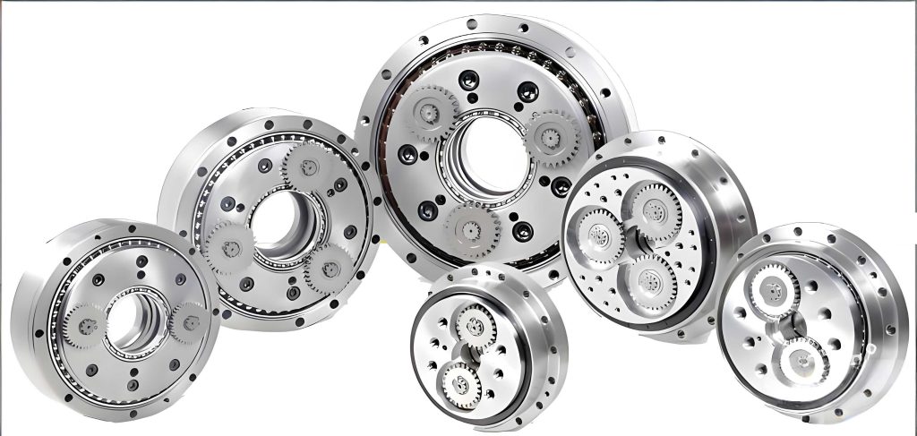
The foundation of the proposed framework is the construction of a comprehensive Digital Twin system for the RV reducer. A DT is more than a simple 3D model; it is a dynamic, data-driven virtual counterpart that mirrors the life-cycle of its physical entity. The developed system architecture is structured into three primary layers: the Information Interaction Layer, the Data Layer, and the Application Service Layer. The physical model of the RV reducer, encompassing its precise geometric dimensions and kinematic relationships, serves as the blueprint. A detailed virtual model of the reducer and its accompanying test rig is then constructed using 3D modeling software. After optimization for computational efficiency and visual fidelity, this model is integrated into a real-time visualization environment, forming the interactive component of the twin.
The true power of the Digital Twin for the RV reducer is unlocked through bi-directional data communication. Vibration sensors are strategically mounted on the reducer’s casing to capture dynamic signals, particularly from the planetary gear stage which is a common failure point. This raw data undergoes preprocessing—filtering, normalization, and formatting—before being stored in a centralized database. This database acts as the Data Layer, harmonizing real-time sensor streams with historical records and simulated fault data. Using standard network protocols like TCP/IP, this processed data is fed to the virtual model. The real-time sensor data drives the animations and state representations of the virtual RV reducer, achieving synchronization between the physical and digital realms. This continuous flow ensures the twin is not a static snapshot but a living model reflecting the current operating conditions of the actual RV reducer.
With a synchronized Digital Twin providing a contextualized data stream, the focus shifts to the intelligent diagnosis core. The Backpropagation Neural Network is chosen for its proven ability to model complex, non-linear relationships inherent in mechanical fault signatures. A standard BP network consists of an input layer, one or more hidden layers, and an output layer. The forward propagation process for our RV reducer diagnosis model can be summarized as follows. For a hidden layer node $i$, its output $q_i$ is calculated using the hyperbolic tangent activation function:
$$q_i = \text{Tanh}\left( \sum_{j=1}^{m} x_j w_{ij} + \beta_i \right)$$
where $x_j$ represents the $j$-th input feature from the preprocessed RV reducer vibration signal, $w_{ij}$ is the weight connecting input $j$ to hidden node $i$, and $\beta_i$ is the bias for node $i$.
The output layer node $k$, corresponding to a specific fault class for the RV reducer, uses the Softmax function for multi-class classification:
$$y_k = \text{Softmax}\left( \sum_{i=1}^{n} q_i \cdot v_{ki} + \lambda_k \right)$$
where $v_{ki}$ is the weight from hidden node $i$ to output node $k$, and $\lambda_k$ is the output layer bias.
The network learns by minimizing a loss function, typically the Mean Squared Error (MSE) between the predicted output $y_k$ and the true label $\hat{y}_k$:
$$\text{Loss} = \frac{1}{K}\sum_{k=1}^{K} (\hat{y}_k – y_k)^2$$
where $K$ is the number of output classes (fault types).
However, traditional BP algorithms are prone to slow convergence and getting trapped in local minima. To overcome these drawbacks and enhance the diagnostic performance for the RV reducer, the Adaptive Moment Estimation (Adam) optimizer is integrated. Adam combines the advantages of two other extension algorithms, AdaGrad and RMSProp, by computing adaptive learning rates for each parameter. It maintains exponentially decaying averages of past gradients ($m_t$, the first moment) and past squared gradients ($v_t$, the second moment). The parameter update rule at iteration $t$ is:
$$m_t = \beta_1 m_{t-1} + (1-\beta_1) \nabla_\theta J(\theta)$$
$$v_t = \beta_2 v_{t-1} + (1-\beta_2) (\nabla_\theta J(\theta) \odot \nabla_\theta J(\theta))$$
$$\hat{m}_t = \frac{m_t}{1-\beta_1^t}, \quad \hat{v}_t = \frac{v_t}{1-\beta_2^t}$$
$$\theta_{t+1} = \theta_t – \frac{\eta}{\sqrt{\hat{v}_t} + \epsilon} \hat{m}_t$$
Here, $\nabla_\theta J(\theta)$ is the gradient of the loss function with respect to parameters $\theta$, $\eta$ is the learning rate, $\beta_1, \beta_2$ are decay rates, and $\epsilon$ is a small constant for numerical stability. This adaptive adjustment of learning rates for each weight and bias in the network significantly accelerates training and improves convergence reliability for the RV reducer fault diagnosis model. Furthermore, an early stopping mechanism is employed to halt training when performance on a validation set ceases to improve, effectively preventing overfitting.
The overall diagnostic workflow is a closed-loop process. Real-time vibration data from the physical RV reducer is fed into the optimized BP network via the Digital Twin’s data pipeline. The network outputs a fault classification. Simultaneously, simulation models within the DT can generate data for known fault modes. A consistency check between the model’s diagnosis and expected behavior (from simulation or historical patterns) can trigger a feedback mechanism. If a significant, unexplained discrepancy is detected, it may indicate a novel fault condition or model drift. This feedback can be used to flag the event for expert analysis and potentially initiate an automated retraining cycle for the neural network with the newly incorporated data, thus enabling continuous learning and adaptation of the diagnostic system for the RV reducer.
To validate the proposed framework, an experimental study was conducted using an RV-80E-56 type reducer. The test rig comprised the reducer, a drive motor, an accelerometer for vibration acquisition, and a data acquisition system. The reducer was operated at a constant speed of 1200 RPM. Vibration data was collected for five distinct states of the planetary gear: healthy, tooth tip crack, broken tooth, tooth root crack, and tooth surface wear. The raw time-domain signals required substantial preprocessing to be suitable for neural network training. The key steps are summarized in the table below:
| Preprocessing Step | Description | Purpose |
|---|---|---|
| 1. Data Cleansing | Identification and imputation of missing/abnormal values using median. | Ensure data integrity and consistency. |
| 2. Normalization | Min-Max scaling to range [0, 1]: $x’ = \frac{x – x_{min}}{x_{max} – x_{min}}$ | Standardize feature scales for stable NN training. |
| 3. Feature Extraction | Calculation of statistical time-domain features from raw signal. | Convert raw waveform into descriptive parameters. |
| 4. Labeling | Assigning integer labels (1 to 5) to each fault class. | Provide ground truth for supervised learning. |
| 5. Dataset Splitting | Random split of 500 samples into training (80%) and testing (20%) sets. | Enable model training and unbiased evaluation. |
The choice of input features is critical. For the RV reducer’s vibration signal, seven time-domain statistical features were selected for their ability to capture changes in amplitude, energy, and waveform shape due to different fault types. These features are listed in the following table:
| Feature Name | Formula | Physical Interpretation |
|---|---|---|
| Mean | $\bar{x} = \frac{1}{N}\sum_{i=1}^{N} x_i$ | Average signal level. |
| Standard Deviation | $\sigma = \sqrt{\frac{1}{N}\sum_{i=1}^{N} (x_i – \bar{x})^2}$ | Signal variability or dispersion. |
| Root Mean Square (RMS) | $X_{RMS} = \sqrt{\frac{1}{N}\sum_{i=1}^{N} x_i^2}$ | Energy content of the signal. |
| Energy | $E = \sum_{i=1}^{N} x_i^2$ | Total signal power. |
| Impulse Factor | $I_f = \frac{\max(|x|)}{\frac{1}{N}\sum_{i=1}^{N} |x_i|}$ | Sensitivity to impulse peaks. |
| Margin Factor | $M_f = \frac{\max(|x|)}{(\frac{1}{N}\sum_{i=1}^{N} \sqrt{|x_i|})^2}$ | Sensitivity to impact faults. |
| Shape Factor | $S_f = \frac{X_{RMS}}{\frac{1}{N}\sum_{i=1}^{N} |x_i|}$ | Waveform shape characteristic. |
The dataset composition after splitting is detailed below, ensuring a balanced representation of fault classes for the RV reducer in both training and testing phases:
| Fault Type (RV Reducer Planet Gear) | Label | Training Samples | Testing Samples |
|---|---|---|---|
| Healthy | 1 | 75 | 25 |
| Tooth Tip Crack | 2 | 80 | 20 |
| Broken Tooth | 3 | 79 | 21 |
| Tooth Root Crack | 4 | 79 | 21 |
| Tooth Surface Wear | 5 | 87 | 13 |
The structure of the BP network was configured with 7 input nodes (for the 7 features), 1 hidden layer, and 5 output nodes (for the 5 fault classes). The optimal number of neurons in the hidden layer was determined empirically by evaluating the Mean Squared Error (MSE) for different sizes. The analysis showed that a hidden layer with 12 neurons yielded the lowest MSE, establishing this as the optimal configuration for diagnosing the RV reducer faults under these conditions. The learning rate was set to 0.01, and the Adam optimizer’s parameters were kept at their default recommended values ($\beta_1=0.9$, $\beta_2=0.999$, $\epsilon=10^{-8}$).
The performance of the optimized Adam-BP neural network was evaluated using standard classification metrics. The diagnosis accuracy on the training set reached 96.5%, while the accuracy on the independent test set was 96%. This high test accuracy demonstrates the model’s excellent generalization capability and its effectiveness in correctly classifying unseen fault conditions of the RV reducer. To benchmark the performance, the Adam-BP model was compared against two other popular neural network models, Generalized Regression Neural Network (GRNN) and Radial Basis Function (RBF) network, using the same RV reducer dataset. The comparative results across key metrics are presented below:
| Performance Metric | Formula | Adam-BP Network | GRNN | RBF Network |
|---|---|---|---|---|
| Accuracy | $\frac{TP+TN}{Total}$ | 96.0% | 90.0% | 86.0% |
| Precision (Macro Avg) | $\frac{TP}{TP+FP}$ | 0.962 | 0.901 | 0.872 |
| Recall (Macro Avg) | $\frac{TP}{TP+FN}$ | 0.961 | 0.902 | 0.868 |
| F1-Score (Macro Avg) | $2 \times \frac{Precision \times Recall}{Precision + Recall}$ | 0.961 | 0.901 | 0.869 |
As the table clearly indicates, the proposed Adam-optimized BP network outperformed both the GRNN and RBF models across all evaluated metrics for the RV reducer fault diagnosis task. The superior accuracy, coupled with high precision and recall scores, confirms that the combination of adaptive gradient-based optimization and appropriate network architecture is highly effective in learning the complex patterns associated with different gear faults in the RV reducer. The Digital Twin framework plays a crucial supporting role in this process by ensuring a steady, contextualized flow of high-quality, synchronized data from the physical system to the diagnostic algorithm.
In conclusion, this research successfully developed and validated an integrated fault diagnosis framework for RV reducers that merges the real-time contextual awareness of a Digital Twin with the powerful pattern recognition capabilities of an optimized neural network. The construction of a synchronized Digital Twin provides a dynamic virtual representation of the physical reducer, enabling real-time monitoring and data provisioning. The integration of the Adam optimizer into the BP neural network effectively addressed common training pitfalls, resulting in a robust and accurate diagnostic model. Experimental validation on a real RV reducer test rig confirmed the framework’s efficacy, with the diagnostic model achieving a high classification accuracy of 96% on unseen test data and outperforming alternative neural network models. This work demonstrates a significant step towards intelligent, predictive maintenance for critical robotic components. Future work will focus on enhancing the framework’s robustness under variable operating conditions, integrating more diverse sensor modalities (e.g., temperature, acoustic emission), and exploring deep learning architectures for automatic feature learning directly from the raw time-series or frequency-domain data provided by the RV reducer’s Digital Twin.