
I investigate the dynamic behavior of a six-degree-of-freedom industrial robot by combining a multi-posture model with the poly-reference least squares complex frequency-domain (pLSCF) method. The motivation is straightforward: the operational accuracy, stability, and reliability of an industrial robot are strongly influenced by its low-order modal parameters, including natural frequencies, damping ratios, and mode shapes. Unlike a single fixed structure, an industrial robot changes its configuration continuously during task execution. Each joint rotation modifies the equivalent mass distribution, stiffness path, and inertial coupling. As a result, the modal parameters of an industrial robot are not constant; they are posture-dependent and often exhibit pronounced multi-joint coupling. This posture dependence is particularly important for high-speed operations, payload handling, and precision tasks such as drilling, milling, and assembly.
Modal analysis is a standard tool for characterizing structural dynamics. For an industrial robot, the governing vibration equation for a given joint configuration can be written as
$$ M(q)\ddot{x}(t) + C(q)\dot{x}(t) + K(q)x(t) = 0 $$
where \(q = [q_1, q_2, \ldots, q_6]^T\) denotes the vector of joint angles, \(M(q)\) is the configuration-dependent mass matrix, \(C(q)\) is the damping matrix, and \(K(q)\) is the stiffness matrix. Neglecting damping for the eigenvalue problem, the modal equation for the \(i\)-th mode becomes
$$ \left[ K(q) – \omega_i^2 M(q) \right] \phi_i = 0 $$
Here, \(\omega_i\) is the \(i\)-th natural angular frequency and \(\phi_i\) is the corresponding mode shape. Because \(M(q)\) and \(K(q)\) vary with \(q\), both \(\omega_i\) and \(\phi_i\) vary with the posture of the industrial robot. This variation is the central challenge that I address in this study.
Existing modal studies on industrial robots often focus on a limited number of postures or a single structural component, such as a joint, a reducer, or a large arm. While these studies provide valuable insight, they do not fully capture the coupled behavior of the complete industrial robot under different configurations. In addition, weak responses and closely spaced modes can make parameter identification unstable when only a single reference is used. To overcome these limitations, I adopt a multi-posture modeling strategy and use pLSCF for modal identification. The pLSCF method exploits multiple reference excitations, allowing strong response channels to compensate for weak response channels and reducing the influence of local noise and joint nonlinearity. Therefore, it is well suited to the posture-dependent and multi-joint coupled dynamics of an industrial robot.
The remainder of this article is organized as follows. I first describe the theoretical basis of the pLSCF algorithm, including basic parameter estimation and mode shape estimation. I then define the multi-posture model, including the two boundary postures and the intermediate postures used for verification. Next, I present the modal experiments, including the excitation methods, measurement points, and signal processing settings. I then report the identified modal parameters, compare the two boundary postures, and analyze the modal assurance criterion (MAC) matrices. Finally, I discuss the physical interpretation of the results and outline future work for dynamic modeling and structural optimization of industrial robots.
Theoretical Basis of pLSCF for Industrial Robots
The pLSCF method represents the frequency response function (FRF) of a linear time-invariant system using a right matrix fraction description. For an industrial robot with \(N_o\) output channels and \(N_i\) input references, the FRF matrix \(H(\omega) \in \mathbb{C}^{N_o \times N_i}\) can be written as
$$ H(\omega) = B(\omega) A^{-1}(\omega) $$
where \(A(\omega)\) and \(B(\omega)\) are denominator and numerator polynomial matrices, respectively. In the pLSCF formulation, the polynomials are expressed in terms of the discrete frequency variable \(\Omega_f\). The numerator and denominator matrices are
$$ B(\Omega_f) = \sum_{j=0}^{n} \beta_j \Omega_f^j, \qquad A(\Omega_f) = \sum_{j=0}^{n} \alpha_j \Omega_f^j $$
Here, \(n\) is the model order, \(\beta_j \in \mathbb{C}^{N_o \times N_i}\) are numerator coefficient matrices, and \(\alpha_j \in \mathbb{C}^{N_i \times N_i}\) are denominator coefficient matrices. The denominator coefficients are usually normalized so that the highest-order coefficient is the identity matrix. The model order \(n\) determines the maximum number of identifiable modes. Because the polynomial coefficients are real, one can identify up to \(n/2\) complex conjugate mode pairs.
For each output channel \(o\) and each frequency line \(f\), the weighted residual is defined as
$$ \varepsilon_{o,f} = w_{o,f} \left( \sum_{j=0}^{n} \beta_{o,j} \Omega_f^j – \sum_{j=0}^{n} \alpha_j \Omega_f^j H_{o,f} \right) $$
where \(H_{o,f}\) is the measured FRF, and \(w_{o,f}\) is an optional weighting factor. The weighting factor can be selected according to the uncertainty of the FRF. In my experiments, I use coherence-based weighting to reduce the influence of frequency regions with poor signal-to-noise ratio. The cost function is then formed as
$$ \ell = \sum_{o=1}^{N_o} \sum_{f=1}^{N_f} \varepsilon_{o,f}^H \varepsilon_{o,f} $$
Minimizing this cost function with respect to the polynomial coefficients leads to a linear least-squares problem. After solving for the denominator coefficients, one constructs the companion matrix and performs an eigenvalue decomposition. The discrete-time poles are obtained from the eigenvalues of the companion matrix. These poles are then converted to continuous-time poles using
$$ \lambda_r = \frac{\ln(z_r)}{T_s} $$
where \(z_r\) is the \(r\)-th discrete-time pole and \(T_s\) is the sampling period. The damped natural frequency \(f_r\) and damping ratio \(\zeta_r\) are obtained from
$$ f_r = \frac{|\lambda_r|}{2\pi}, \qquad \zeta_r = -\frac{\operatorname{Re}(\lambda_r)}{|\lambda_r|} $$
To distinguish physical poles from computational poles, I use a stabilization diagram. The stability criteria are based on the relative variation of natural frequency, damping ratio, and mode shape between successive model orders. In this study, I use the following thresholds:
$$ \frac{|f_i – f_{i-1}|}{f_i} < 0.008, \qquad \frac{|\zeta_i – \zeta_{i-1}|}{\zeta_i} < 0.04, \qquad \mathrm{MAC}(\phi_i, \phi_{i-1}) > 0.95 $$
These thresholds are stricter than the common values of 1%, 5%, and 0.90. The reason is that the FRF data quality in my experiments is high, and a stricter criterion helps eliminate spurious poles that may appear near weakly excited modes. The stabilization diagram is constructed by repeating the pLSCF identification for increasing model orders. Poles that appear repeatedly at consecutive orders and align with peaks in the FRF are selected as physical poles. Other poles are discarded as numerical or noise poles.
After the poles and participation vectors are obtained, the mode shapes are estimated in a second least-squares step. For an acceleration FRF, the modal model can be written as
$$ H(\omega_f) = \sum_{r=1}^{N_m} \left( \frac{\phi_r L_r^T}{j\omega_f – \lambda_r} + \frac{\phi_r^* L_r^H}{j\omega_f – \lambda_r^*} \right) + \rho_l + \rho_u \omega_f^2 $$
where \(\phi_r\) is the \(r\)-th mode shape, \(L_r\) is the \(r\)-th participation vector, \(N_m\) is the number of modes retained in the analysis band, \(\rho_l\) is the lower residual term, and \(\rho_u\) is the upper residual term. The lower residual accounts for modes below the analysis band, while the upper residual accounts for modes above the analysis band. The superscript \(*\) denotes complex conjugation, and the superscript \(H\) denotes Hermitian transpose. Because the participation vectors are already normalized in the first step, the mode shapes are uniquely determined by the second least-squares solution.
The linear system for mode shape estimation can be written in compact form as
$$ h = A X $$
where \(h\) is the observation vector containing the real and imaginary parts of the measured FRFs, \(A\) is the coefficient matrix, and \(X\) is the vector of unknown mode shape components and residual terms. The solution is obtained using the Moore–Penrose pseudoinverse:
$$ X = A^{\dagger} h $$
For the solution to be well conditioned, the number of frequency lines must satisfy \(2N_f > 2N_m + 4N_i\). In my experiments, the number of frequency lines is 3200, which is far larger than the number of retained modes and references. Therefore, the least-squares problem is strongly overdetermined and numerically stable.
Multi-Posture Model of the Industrial Robot
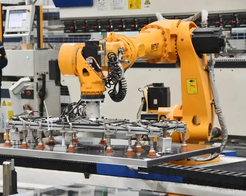
The experimental object is a six-degree-of-freedom industrial robot with a payload capacity of 70 kg and a reach of 2100 mm. The robot consists of a base, a shoulder, a large arm, an elbow, a small arm, and a wrist. Each joint rotates about its axis, allowing the industrial robot to achieve different working postures. The base is mounted on a steel base plate, which is fixed to a concrete floor. Eight M20 bolts are used to connect the base, and they are tightened in stages with a specified preload torque.
Because the dynamic behavior of an industrial robot depends on its joint configuration, I define two boundary postures and three intermediate postures. The two boundary postures are chosen to represent a near-base bending configuration and a far-reach stretching configuration. The joint angles and end-effector positions are summarized in Table 1.
| Model | Joint angles \(q\) (deg) | End-effector position (mm) | Description |
|---|---|---|---|
| Model 1 | [0, -90, 90, 0, 0, 0] | (1400, 0, 1500) | Near-base bending posture; compact configuration; strong joint coupling |
| Model 2 | [0, -50, 60, 0, 0, 0] | (2000, 0, 1000) | Far-reach stretching posture; horizontal extension; lower overall stiffness |
| Model 3 | [0, -80, 82.5, 0, 0, 0] | Intermediate | Intermediate posture along the joint-angle path |
| Model 4 | [0, -70, 75, 0, 0, 0] | Intermediate | Intermediate posture along the joint-angle path |
| Model 5 | [0, -60, 67.5, 0, 0, 0] | Intermediate | Intermediate posture along the joint-angle path |
For the two boundary postures, I build simplified finite element models that retain the main load-carrying structure and the primary connection relationships. Small features such as cables, bolts, and small flanges are ignored because their contributions to the low-order modes are limited. The simplification is based on the spatial sampling principle: I retain enough measurement points to describe the amplitude and phase variation of the target mode shapes along the main structural paths. The number of measurement points is determined by the spatial complexity of the target modes. For Model 1, the posture is compact and the vibration field is more complex, so I use 37 measurement points. For Model 2, the posture is extended and the low-order modes are dominated by global cantilever bending, so 12 measurement points are sufficient. The distribution of measurement points is given in Table 2.
| Model | Base | Large arm | Small arm | Wrist | Total |
|---|---|---|---|---|---|
| Model 1 | 12 | 12 | 8 | 5 | 37 |
| Model 2 | 1 | 4 | 2 | 5 | 12 |
The measurement point layout follows three principles: axial sampling, circumferential coverage, and avoidance of modal nodes. Along the large arm and small arm, points are distributed uniformly in the axial direction. Near the elbow and wrist, where stiffness changes abruptly, the point density is increased. For Model 1, points are also placed at different circumferential positions to distinguish bending and torsional responses. For Model 2, the dominant response is in-plane bending, so points are concentrated along the robot axis and the flexibility direction, with additional coverage at the elbow and the end effector. Candidate points are evaluated by comparing FRF amplitudes and coherence functions. Fixed reference points are chosen so that they are not located near the nodes of the first three modes. Under the condition that the mode shape matrix has full column rank, the number of effective spatial degrees of freedom should be no less than the number of target modes. Both 37 and 12 measurement points satisfy this requirement for the first three modes.
The experimental system is shown below.
Modal Experiments on the Industrial Robot
I use two excitation methods: impact hammer testing and shaker testing. Impact hammer testing has the advantages of a wide frequency band and simple implementation. It is suitable for structures with high stiffness, stable boundary conditions, and sufficient impact energy. However, for flexible structures with pronounced low-frequency response, impact hammer testing can be affected by double hits, force fluctuations, and transient displacement. Shaker testing provides continuous excitation with stable amplitude and spectrum. It is suitable for flexible structures with strong low-order response, but the push rod, added mass, and shaker attachment can influence the boundary conditions. Therefore, I select the excitation method according to the stiffness and response characteristics of each posture. For Model 1, the structure is compact and stable, so impact hammer testing is used. For Model 2, the end-effector region has large flexibility and high vibration amplitude, so a shaker is used to apply burst random excitation in the horizontal direction.
The measurement chain includes an eight-channel data acquisition and analysis instrument with 24-bit resolution and a maximum sampling rate of 204.8 kHz, a force hammer with a hard nylon tip, an electrodynamic shaker with a rated force of 100 N, a modal analysis software package, and IEPE-type triaxial accelerometers. Each accelerometer has a mass of about 10 g and is attached to the measurement point with wax. The added mass effect on the natural frequencies of the industrial robot is negligible.
The analysis band is set to 0–400 Hz. The sampling frequency is 2048 Hz, and the number of FFT lines is 3200, which gives a frequency resolution of 0.125 Hz. This resolution is much smaller than the minimum spacing between adjacent modes, which is about 5 Hz. For the shaker test, a burst random signal with a duty cycle of 80% is used, and each record length is 8 s. For the impact hammer test, the measured force pulse width is about 1.8 ms with no obvious decay. The impact hammer test is averaged over 5 independent impacts, while the shaker test is averaged over 30 independent records. The coherence function is required to be higher than 0.95 near the resonance peaks, and the coefficient of variation of the identified natural frequencies in repeated tests is required to be less than 1.4%. The experimental settings are summarized in Table 3.
| Parameter | Value |
|---|---|
| Analysis band | 0–400 Hz |
| Sampling frequency | 2048 Hz |
| Number of FFT lines | 3200 |
| Frequency resolution | 0.125 Hz |
| Excitation for Model 1 | Impact hammer, 5 averages |
| Excitation for Model 2 | Shaker, burst random, 30 averages |
| Coherence threshold | > 0.95 near resonance |
| Frequency variation threshold | < 1.4% in repeated tests |
To verify reciprocity, I select representative measurement point pairs, such as base–large arm and elbow–wrist. I exchange the excitation and response points and compare the FRFs \(H_{i,j}\) and \(H_{j,i}\). The normalized reciprocity error is defined as
$$ \varepsilon_H = \frac{\| H_{i,j} – H_{j,i} \|_2}{\| H_{i,j} \|_2} \times 100\% $$
The measured reciprocity error is below 5%. In addition, I compare the first three natural frequencies, damping ratios, and mode shapes obtained from hammer testing and shaker testing for the same posture. The correlation coefficient of reciprocal FRFs is no less than 0.95, the natural frequency deviation is no more than 0.8%, and the damping ratio deviation is no more than 5%. These results indicate that the two excitation methods produce consistent modal parameters for the industrial robot.
I also evaluate the influence of sensor mass and excitation position offset. The maximum shift of the first three natural frequencies caused by sensor added mass is about 0.1 Hz, and the maximum relative change of damping ratio is about 2.8%. When the excitation position is shifted by 3 mm, the maximum relative changes of natural frequency and damping ratio are about 0.2 Hz and 4.6%, respectively. The background noise root mean square value is less than 1% of the effective response root mean square value when the industrial robot is stationary. Therefore, the experimental results have good repeatability and credibility.
Modal Parameter Identification Results
I collect the excitation and response signals for the multi-posture model, transform them into the frequency domain using FFT, and compute the FRFs. The pLSCF method is then used to fit the FRFs. The FRF is represented as a rational fraction:
$$ H(s) = \frac{B(s)}{A(s)} $$
where \(A(s)\) and \(B(s)\) are the denominator and numerator polynomials, and \(s = j\omega\) is the complex frequency variable. The error between the theoretical model and the measured function is minimized:
$$ J = \sum_{k=1}^{N_f} \left\| A(j\omega_k) H(j\omega_k) – B(j\omega_k) \right\|_2^2 $$
By solving this optimization problem, I obtain the system poles, which contain the natural frequency and damping information. The stabilization diagrams for the two boundary postures are constructed by repeating the identification for increasing model orders. Poles that satisfy the stability criteria, form a vertical stable sequence, and align with FRF peaks are selected as physical poles. The remaining poles are discarded.
The identified first three modal parameters for Model 1 and Model 2 are listed in Table 4. The damping ratios of both postures range from 0.968% to 1.745%.
| Model | Mode 1 frequency (Hz) | Mode 1 damping ratio (%) | Mode 2 frequency (Hz) | Mode 2 damping ratio (%) | Mode 3 frequency (Hz) | Mode 3 damping ratio (%) |
|---|---|---|---|---|---|---|
| Model 1 | 14.635 | 0.968 | 40.637 | 1.446 | 44.131 | 1.511 |
| Model 2 | 13.365 | 1.346 | 49.266 | 1.745 | 52.029 | 1.440 |
The relative frequency changes between the two boundary postures are calculated as
$$ \Delta f_i = \frac{f_{i,\text{Model 2}} – f_{i,\text{Model 1}}}{f_{i,\text{Model 1}}} \times 100\% $$
The results are given in Table 5. Compared with Model 1, the first natural frequency of Model 2 decreases by 8.68%, while the second and third natural frequencies increase by 21.23% and 17.90%, respectively.
| Mode | Model 1 frequency (Hz) | Model 2 frequency (Hz) | Relative change (%) |
|---|---|---|---|
| First | 14.635 | 13.365 | -8.68 |
| Second | 40.637 | 49.266 | +21.23 |
| Third | 44.131 | 52.029 | +17.90 |
The mode shapes are also extracted from the pLSCF identification. The first mode of both postures is dominated by large-arm swing in the direction perpendicular to the base axis. The second and third modes mainly involve small-arm bending. In Model 1, the center of mass of the industrial robot is closer to the base, the equivalent rotational inertia is smaller, and the large-arm support stiffness is relatively high. Therefore, the first natural frequency is slightly higher than that of Model 2. In Model 2, the small arm is extended, and the second and third mode shapes are more concentrated in the small-arm region. The equivalent participating mass is reduced, and the joint angle change increases the equivalent constraint stiffness in the bending direction. These two effects together cause the second and third natural frequencies to increase.
The damping ratios of the two postures remain within a small range, from 0.968% to 1.745%. This indicates that posture change has a weaker influence on damping than on natural frequency. When the industrial robot extends, the gravity arm increases, which changes the contact load and micro-slip state of the shoulder, elbow, and wrist transmission pairs. This in turn alters joint friction energy dissipation. However, material internal damping and transmission preload remain nearly unchanged. Therefore, the damping ratio only fluctuates slightly and does not show a clear monotonic trend.
Modal Assurance Criterion Analysis
To evaluate the similarity between mode shapes, I calculate the modal assurance criterion (MAC) between the identified mode shape matrix \(\Phi\) and the reference or simulation mode shape matrix \(\Psi\). The MAC value between the \(i\)-th and \(j\)-th modes is defined as
$$ \mathrm{MAC}_{ij} = \frac{|\phi_i^T \psi_j|^2}{(\phi_i^T \phi_i)(\psi_j^T \psi_j)} $$
where \(\phi_i\) and \(\psi_j\) are the \(i\)-th and \(j\)-th mode shape vectors. The MAC matrix is assembled from all mode pairs. A MAC value close to 1 indicates high similarity, while a value close to 0 indicates low similarity. For a well-identified modal model, the diagonal MAC values should be close to 1, and the off-diagonal MAC values should be as small as possible.
The MAC matrices for Model 1 and Model 2 are given in Table 6 and Table 7, respectively. For Model 1, all off-diagonal MAC values are below 0.06. For Model 2, the MAC value between the first and second modes is 0.18, while all other off-diagonal MAC values are below 0.07. This indicates that the mode shapes generally have good spatial independence.
| Model 1 MAC | Mode 1 | Mode 2 | Mode 3 |
|---|---|---|---|
| Mode 1 | 1.00 | 0.05 | 0.03 |
| Mode 2 | 0.05 | 1.00 | 0.06 |
| Mode 3 | 0.03 | 0.06 | 1.00 |
| Model 2 MAC | Mode 1 | Mode 2 | Mode 3 |
|---|---|---|---|
| Mode 1 | 1.00 | 0.18 | 0.07 |
| Mode 2 | 0.18 | 1.00 | 0.06 |
| Mode 3 | 0.07 | 0.06 | 1.00 |
The higher first–second MAC value of Model 2 indicates that the coupling between the first and second modes is mainly concentrated in the elbow, small arm, and wrist. This coupling arises because the extended posture increases the equivalent rotational inertia at the end effector. At the same time, the joint reducers and bearings have different stiffnesses in the axial, radial, and torsional directions. The configuration change causes some low-stiffness directions to align with the main bending direction of the complete industrial robot, which enhances modal coupling. This coupling can reduce the end-effector dynamic stiffness and increase vibration response in adjacent resonance bands, thereby increasing end-effector pose errors during machining or assembly. However, the MAC value is still much lower than 1, which means that the two modes remain separable.
The stability criteria used in the pLSCF identification are summarized in Table 8. The thresholds are stricter than the commonly used values, which helps to remove spurious poles while preserving physical poles.
| Criterion | Threshold |
|---|---|
| Relative natural frequency error | < 0.8% |
| Relative damping ratio error | < 4% |
| Mode shape MAC between successive orders | > 0.95 |
I also examined the influence of measurement and excitation errors on the modal parameters. The results are listed in Table 9. The maximum frequency shift caused by sensor added mass is about 0.1 Hz, and the maximum damping ratio change is about 2.8%. The maximum frequency and damping ratio changes caused by a 3 mm excitation position offset are about 0.2 Hz and 4.6%, respectively. These values are small compared with the differences between the two boundary postures. Therefore, the identified posture-dependent modal trends are reliable.
| Error source | Maximum frequency change | Maximum damping ratio change |
|---|---|---|
| Sensor added mass | 0.1 Hz | 2.8% |
| Excitation position offset (3 mm) | 0.2 Hz | 4.6% |
For the intermediate postures, the simulation and experimental results show a continuous trend. As the industrial robot extends from Model 1 to Model 2, the first natural frequency gradually decreases, while the second and third natural frequencies generally increase. The damping ratio fluctuates slightly between the results of the two boundary postures. This confirms that the two boundary postures capture the main modal evolution along the selected joint-angle path. The intermediate posture results are summarized in Table 10 as qualitative trends.
| Posture | First frequency trend | Second frequency trend | Third frequency trend | Damping ratio trend |
|---|---|---|---|---|
| Model 1 | Highest | Lowest | Lowest | Lowest |
| Model 3 | Decreasing | Increasing | Increasing | Slight fluctuation |
| Model 4 | Decreasing | Increasing | Increasing | Slight fluctuation |
| Model 5 | Decreasing | Increasing | Increasing | Slight fluctuation |
| Model 2 | Lowest | Highest | Highest | Highest |
Discussion and Physical Interpretation
The results show that the modal parameters of an industrial robot are strongly posture-dependent. The first mode is governed by the large-arm swing, which is sensitive to the distance between the center of mass and the base. In the near-base bending posture, the center of mass is closer to the base, so the equivalent rotational inertia is smaller and the first natural frequency is higher. In the far-reach stretching posture, the center of mass moves farther from the base, the equivalent rotational inertia increases, and the first natural frequency decreases. This explains the 8.68% reduction in the first natural frequency from Model 1 to Model 2.
The second and third modes are governed by small-arm bending and local joint compliance. In the near-base bending posture, the small arm is folded, and the mode shapes involve more of the complete structure. In the far-reach stretching posture, the small arm is extended, and the second and third mode shapes become more concentrated in the small-arm region. The equivalent participating mass decreases, and the joint angle change increases the equivalent bending constraint stiffness. As a result, the second and third natural frequencies increase by 21.23% and 17.90%, respectively. This behavior is consistent with the mode shape observations: the second and third modes in Model 2 have larger amplitudes in the small arm and wrist.
The damping ratio remains within a relatively narrow range. This suggests that the energy dissipation mechanisms in the industrial robot are not strongly affected by posture. The main dissipation sources are material internal damping, joint friction, and transmission preload. When the industrial robot extends, the gravity arm increases, which changes the normal contact load and micro-slip at the shoulder, elbow, and wrist. This changes the friction energy dissipation, but the change is moderate. Therefore, the damping ratio only fluctuates slightly. The absence of a clear monotonic trend indicates that multiple mechanisms compete: some joints may experience increased friction due to higher contact load, while others may experience reduced friction due to geometric changes.
The MAC analysis provides additional insight into modal coupling. For Model 1, the off-diagonal MAC values are all below 0.06, which means that the first three modes are well separated. For Model 2, the first–second MAC value is 0.18, which indicates moderate coupling. The coupling is concentrated in the elbow, small arm, and wrist. This is important for industrial robot applications because the extended posture is often used for large-workspace tasks such as drilling and milling. In these tasks, the end-effector dynamic stiffness is critical. If the first and second modes are coupled, the resonance band becomes broader, and the end-effector vibration may increase. This can reduce machining accuracy and surface quality. Therefore, the coupling information obtained from the MAC matrix can be used to guide structural optimization of the elbow and wrist.
The pLSCF method is particularly effective for this application because it uses multiple references. In the impact hammer test, I use multiple excitation points and multiple response points. In the shaker test, I use a single fixed excitation point but multiple response channels. In both cases, the multi-reference formulation allows strong response channels to compensate for weak response channels. This reduces the influence of local noise and joint nonlinearity. The stabilization diagram also helps to separate physical poles from computational poles. By using stricter stability thresholds, I obtain a clean set of physical poles that correspond to the FRF peaks. This is important for an industrial robot because the low-order modes may be closely spaced, especially in the extended posture.
The experimental results also confirm the reciprocity of the FRFs. The reciprocity error is below 5%, which indicates that the system behaves approximately linearly and time-invariantly within the small-amplitude vibration range. The sensor added mass and excitation position offset have small effects on the identified modal parameters. The background noise is low. Therefore, the measured posture-dependent modal trends are reliable and can be used for dynamic modeling of the industrial robot.
Implications for Dynamic Modeling and Optimization
The identified modal parameters provide a foundation for dynamic modeling of the industrial robot. Because the modal parameters vary with posture, a single fixed modal model is not sufficient for accurate prediction of the dynamic behavior across the workspace. Instead, the joint-angle path can be used to interpolate the modal parameters between the boundary postures. The two boundary postures serve as boundary samples in joint space. Additional intermediate postures can be added along the joint-angle path to build a continuous mapping from joint angles and payload to modal parameters. This mapping can be written conceptually as
$$ \left( f_i, \zeta_i, \phi_i \right) = \mathcal{F}(q, m_p) $$
where \(q\) is the joint angle vector and \(m_p\) is the payload. The mapping \(\mathcal{F}\) can be constructed using interpolation, polynomial regression, or a Gaussian process. The accuracy of the mapping can be evaluated using postures that are not included in the training set. For future work, I plan to use a frequency prediction error of less than 0.6% and a mode shape MAC greater than 0.98 as acceptance criteria.
The MAC results also provide targets for structural optimization. The first–second MAC value of Model 2 is 0.18, and the coupling is concentrated in the elbow and wrist. To reduce this coupling, the stiffness distribution of the elbow and wrist can be adjusted. For example, the bearing preload, reducer stiffness, and local rib layout can be modified. The optimization objective can be formulated as
$$ \min_{x} \left( -f_1^{\min} + w_1 \mathrm{MAC}_{12} + w_2 \Delta m \right) $$
where \(f_1^{\min}\) is the minimum first natural frequency over the workspace, \(\mathrm{MAC}_{12}\) is the first–second modal coupling, \(\Delta m\) is the mass increment, and \(w_1\) and \(w_2\) are weighting factors. The optimization is subject to constraints on stiffness, strength, and geometric compatibility. After optimization, the same modal experiments can be performed to verify the improvement.
In addition, the dynamic stiffness of the industrial robot can be predicted from the identified modal parameters. For a given posture and payload, the FRF at the end effector can be reconstructed as
$$ H_{\text{end}}(\omega) = \sum_{r=1}^{N_m} \left( \frac{\phi_r^{\text{end}} L_r^T}{j\omega – \lambda_r} + \frac{\phi_r^{\text{end}*} L_r^H}{j\omega – \lambda_r^*} \right) + \rho_l + \rho_u \omega^2 $$
where \(\phi_r^{\text{end}}\) is the end-effector component of the \(r\)-th mode shape. This reconstructed FRF can be used to evaluate the dynamic stiffness at the tool center point. It can also be used to select task postures that avoid resonance bands. For example, if the dominant excitation frequency of a machining process is close to the first natural frequency, the posture can be adjusted to shift the natural frequency away from the excitation frequency. This is a practical way to improve machining stability and surface quality.
Conclusion
I have presented a modal analysis method for industrial robots based on a multi-posture model and the pLSCF method. The method is applied to a six-degree-of-freedom industrial robot with two boundary postures and several intermediate postures. The main conclusions are as follows.
First, the dynamic behavior of the industrial robot is strongly posture-dependent. Compared with the near-base bending posture, the far-reach stretching posture has a first natural frequency that is 8.68% lower, while the second and third natural frequencies are 21.23% and 17.90% higher. The damping ratios of both postures remain within 0.968%–1.745%.
Second, the pLSCF method with multiple references provides stable identification of the first three modes. The stabilization diagram, together with strict stability criteria, effectively separates physical poles from computational poles. The mode shapes are consistent with the physical interpretation: the first mode is dominated by large-arm swing, and the second and third modes are dominated by small-arm bending.
Third, the MAC analysis shows good spatial independence for most modes. For the near-base bending posture, all off-diagonal MAC values are below 0.06. For the far-reach stretching posture, the first–second MAC value is 0.18, and all other off-diagonal values are below 0.07. The coupling in the extended posture is concentrated in the elbow and wrist, which suggests that these regions should be considered in structural optimization.
Fourth, the experimental results are reliable. Reciprocity errors are below 5%, sensor added mass effects are small, and the background noise is low. The identified modal parameters provide a reliable basis for dynamic modeling and analysis of industrial robots.
For future work, I plan to extend the multi-posture model to include additional intermediate postures and payload conditions. I will build a mapping from joint angles and payload to modal parameters, and I will validate the mapping using postures that are not used in the modeling. I will also use finite element model updating to identify equivalent joint stiffness and damping. Finally, I will perform structural optimization of the elbow and wrist with the objectives of increasing the minimum first natural frequency over the workspace, improving end-effector dynamic stiffness, reducing the first–second modal coupling MAC value, and limiting mass increment. The optimized design will be verified by modal experiments under the same postures.
The proposed method is not limited to the specific industrial robot tested in this study. It can be applied to other multi-joint industrial robots, as well as to other flexible mechanisms with posture-dependent dynamics. The combination of a multi-posture model, multiple-reference excitation, and pLSCF identification provides a practical and robust framework for characterizing the dynamic behavior of industrial robots in real operating conditions.