
1. Introduction and Research Background
In the evolution of robotics, wheeled and tracked platforms initially broke through traditional design constraints, paving the way for modern robotics. With the continuous development of bionics, legged robots have progressively evolved toward simulating biological motion mechanisms. Bipedal and quadrupedal robots, mimicking the locomotion of birds and mammals respectively, have demonstrated significant advantages in traversing uneven terrain and efficient load transportation. Today, robots are increasingly advancing toward higher levels of anthropomorphism.
Under the strategic framework of national initiatives, highly anthropomorphic robots exhibit superior flexibility and adaptability in collaborative, assembly, and maintenance tasks. However, providing sufficient human motion data suitable for embodied robot remains a critical challenge for anthropomorphic motion control and action learning. Due to differences in human topology, mass distribution, and kinematic constraints compared to robots, raw human motion data cannot be directly applied to drive embodied robot, severely limiting the realization of anthropomorphic behavior.
This dissertation addresses these challenges through two primary contributions. First, I propose a human motion data segmentation and synthesis technique that achieves effective reuse of limited data, constructing a human motion dataset suitable for embodied robot imitation. Second, I develop an action mapping and retargeting method based on human motion data that addresses the accuracy and fluency issues existing in current action generation techniques.
2. Embodied Robot System and Kinematic Modeling
2.1 System Description
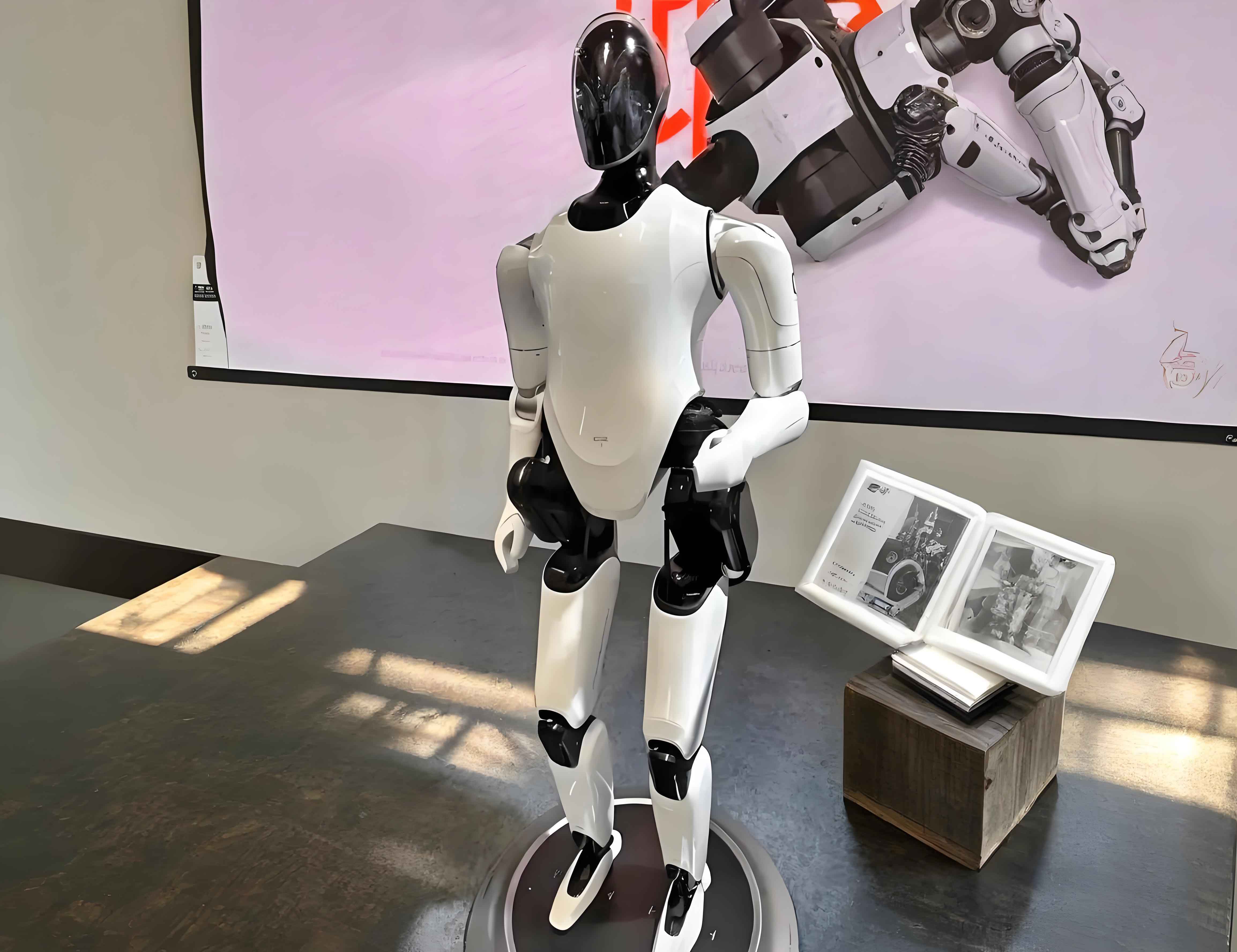
The research platform is a full-size general-purpose embodied robot with a highly biomimetic torso structure. The entire system possesses up to 43 degrees of freedom (DOF), with a maximum joint peak torque of 396 N·m. The robot has an overall height of approximately 1.85 meters and weighs approximately 80 kilograms, demonstrating diverse locomotion capabilities including fast walking, flexible obstacle avoidance, stable slope climbing, and impact disturbance rejection. Table 1 summarizes the DOF configuration of the robot.
| Joint Group | DOF |
|---|---|
| Head | 2 |
| Legs (each) | 6 × 2 |
| Waist | 3 |
| Arms (each) | 7 × 2 |
| Dexterous Hands | 6 × 2 |
2.2 Spatial Transformation Description
In describing the state of an embodied robot in space, both position and orientation must be considered. By establishing coordinate systems on each robot component and describing the transformations between them, the motion relationships can be expressed. Given a point \(^C P\) expressed in coordinate system \(\{C\}\), its expression in coordinate system \(\{A\}\) can be derived through sequential transformations:
\[
^A P = {}^A_B T \cdot {}^B_C T \cdot {}^C P
\tag{2.1}
\]
The composite transformation matrix from \(\{C\}\) to \(\{A\}\) is:
\[
{}^A_C T = {}^A_B T \cdot {}^B_C T
=
\begin{bmatrix}
{}^A_B R \cdot {}^B_C R & {}^A_B R \cdot {}^B P_{C_{ORG}} + {}^A P_{B_{ORG}} \\
0_{1 \times 3} & 1
\end{bmatrix}
\tag{2.2}
\]
The fundamental rotation matrices about the X, Y, and Z axes are:
\[
R_x(\alpha) =
\begin{bmatrix}
1 & 0 & 0 \\
0 & \cos\alpha & -\sin\alpha \\
0 & \sin\alpha & \cos\alpha
\end{bmatrix}, \quad
R_y(\beta) =
\begin{bmatrix}
\cos\beta & 0 & \sin\beta \\
0 & 1 & 0 \\
-\sin\beta & 0 & \cos\beta
\end{bmatrix}
\tag{2.3}
\]
\[
R_z(\gamma) =
\begin{bmatrix}
\cos\gamma & -\sin\gamma & 0 \\
\sin\gamma & \cos\gamma & 0 \\
0 & 0 & 1
\end{bmatrix}
\tag{2.4}
\]
Additionally, quaternions provide an efficient alternative for representing orientation, particularly in motion capture data:
\[
q = w + xi + yj + zk
\tag{2.5}
\]
where \(w, x, y, z \in \mathbb{R}\) and \(i^2 = j^2 = k^2 = ijk = -1\).
2.3 D-H Coordinate System Establishment
The Denavit-Hartenberg (D-H) method provides a standardized approach for kinematic modeling of multi-DOF robots. For the embodied robot under study, the left arm coordinate system transformation chain is established through a series of translations and rotations. The general D-H transformation matrix between consecutive coordinate systems is:
\[
{}_i^{i-1} T =
\begin{bmatrix}
\cos\theta_i & -\sin\theta_i & 0 & a_{i-1} \\
\sin\theta_i \cos\alpha_{i-1} & \cos\theta_i \cos\alpha_{i-1} & -\sin\alpha_{i-1} & -d_i \sin\alpha_{i-1} \\
\sin\theta_i \sin\alpha_{i-1} & \cos\theta_i \sin\alpha_{i-1} & \cos\alpha_{i-1} & d_i \cos\alpha_{i-1} \\
0 & 0 & 0 & 1
\end{bmatrix}
\tag{2.6}
\]
The link parameters are defined in Table 2.
| Parameter | Description |
|---|---|
| \(a_i\) | Distance along \(X_i\) from \(Z_i\) to \(Z_{i+1}\) |
| \(\alpha_i\) | Angle about \(X_i\) from \(Z_i\) to \(Z_{i+1}\) |
| \(d_i\) | Distance along \(Z_i\) from \(X_{i-1}\) to \(X_i\) |
| \(\theta_i\) | Angle about \(Z_i\) from \(X_{i-1}\) to \(X_i\) |
The key link dimensions are provided in Table 3.
| Link Name | Abbreviation | Length (cm) |
|---|---|---|
| Spine | \(d_1\) | 39.22 |
| Clavicle | \(d_2\) | 16.16 |
| Upper Arm 1 | \(d_3\) | 4.10 |
| Upper Arm 2 | \(d_4\) | 12.26 |
| Upper Arm 3 | \(d_5\) | 17.74 |
| Forearm | \(d_6\) | 10.35 |
| Hand | \(d_7\) | 19.65 |
2.4 Forward Kinematics Derivation and Verification
The forward kinematic model establishes the mapping from joint angles to the end-effector pose. For the left arm, the composite transformation is:
\[
{}^0_{19} T = {}^0_1 T \cdot {}^1_2 T \cdot {}^2_3 T \cdot {}^3_4 T \cdot {}^4_5 T \cdot {}^5_6 T \cdots {}^{18}_{19} T
\tag{2.7}
\]
The end-effector position can be expressed as a function of the joint angles:
\[
\begin{cases}
p_x = f_1(\theta_1, \theta_2, \theta_3, \theta_4, \theta_5, \theta_6) \\
p_y = f_2(\theta_1, \theta_2, \theta_3, \theta_4, \theta_5, \theta_6) \\
p_z = f_3(\theta_1, \theta_2, \theta_3, \theta_4, \theta_5, \theta_6)
\end{cases}
\tag{2.8}
\]
The verification process involved comparing end-effector positions computed from the forward kinematic model with those extracted from the three-dimensional animation environment. The results demonstrated centimeter-level consistency, validating the accuracy of the developed kinematic model and establishing a solid foundation for subsequent motion retargeting studies.
2.5 Jacobian Matrix and Workspace Analysis
The Jacobian matrix relates joint-space velocities to end-effector Cartesian velocities:
\[
\dot{X} = J(\theta) \dot{\theta}
\tag{2.9}
\]
where:
\[
J(\theta) =
\begin{bmatrix}
\frac{\partial p_x}{\partial \theta_1} & \frac{\partial p_x}{\partial \theta_2} & \cdots & \frac{\partial p_x}{\partial \theta_n} \\
\frac{\partial p_y}{\partial \theta_1} & \frac{\partial p_y}{\partial \theta_2} & \cdots & \frac{\partial p_y}{\partial \theta_n} \\
\frac{\partial p_z}{\partial \theta_1} & \frac{\partial p_z}{\partial \theta_2} & \cdots & \frac{\partial p_z}{\partial \theta_n}
\end{bmatrix}
\tag{2.10}
\]
The workspace analysis, performed through recursive sampling of joint angle combinations, revealed that the upper limbs exhibit an approximately spherical workspace, enabling uniform motion distribution. The lower limbs demonstrate a hemispherical workspace with certain unreachable regions, which imposes constraints on complex lower-limb movement imitation. The joint motion ranges are summarized in Table 4.
| Joint | Motion Range (degrees) |
|---|---|
| Waist Pitch | −17 to 35 |
| Waist Roll | −40 to 40 |
| Waist Yaw | −45 to 45 |
| Hip Pitch | −77 to 105 |
| Hip Roll | −10 to 25 |
| Hip Yaw | −40 to 40 |
| Knee Pitch | −120 to 5 |
| Ankle Pitch | −30 to 60 |
| Ankle Roll | −25 to 25 |
| Shoulder Pitch | −170 to 170 |
| Shoulder Roll | −105 to 105 |
| Elbow Flexion | 0 to 170 |
| Wrist Pitch | −105 to 105 |
| Wrist Roll | −60 to 60 |
3. Human Motion Data Segmentation and Synthesis Based on Spatio-Temporal Feature Extraction
3.1 Motion Data Acquisition and Preprocessing
For the embodied robot to learn anthropomorphic behaviors, sufficient and diverse human motion data is essential. I utilized two data sources: inertial motion capture suit measurements and the public CMU motion capture database. The motion capture system provides high-precision inertial sensors placed at key body locations, capturing full-body motion at 30-60 Hz.
The raw motion data is stored in BVH format, containing skeletal hierarchy information (HIERARCHY section) and motion sequence data (MOTION section). Each frame includes root joint position, and joint rotations expressed as Euler angles.
The foot positions in the world coordinate system are computed through the kinematic chain:
\[
^O_F P = {}^O_R R \cdot {}^R_B R \cdot {}^B_T R \cdot {}^T_S R \cdot offset_F + {}^O_R R \cdot {}^R_B R \cdot {}^B_T R \cdot offset_S + \cdots
\tag{3.1}
\]
3.2 Dynamic Balance Feature Extraction
To capture the dynamic characteristics of human motion, I formulated a simplified inverted pendulum model connecting the center of mass (COM) to the supporting foot. The pendulum length is computed as:
\[
r = \sqrt{(x_{com} – x_{if})^2 + (z_{com} – z_{if})^2}
\tag{3.2}
\]
The pendulum inclination angle in the sagittal plane is:
\[
\theta = \arctan\left(\frac{z_{com} – z_{if}}{x_{com} – x_{if}}\right)
\tag{3.3}
\]
The COM position is calculated using the weighted average of segment masses:
\[
P_{com} = \frac{\sum m_i \cdot P_i^O}{\sum m_i}
\tag{3.4}
\]
The COM velocity and acceleration are subsequently derived through numerical differentiation:
\[
V_{com} = \frac{dP_{com}}{dt}, \quad A_{com} = \frac{d^2P_{com}}{dt^2}
\tag{3.5}
\]
3.3 Gait Periodic Feature Extraction
Gait parameters provide critical segmentation information. The foot support states (double support, left support, right support, no support) are classified by comparing foot heights against adaptive thresholds. The duty cycle for each frame is:
\[
D_{R_j} = \frac{s_j}{2}
\tag{3.6}
\]
where \(s_j\) represents the number of supporting feet. The averaged duty cycle over a gait cycle is:
\[
D = \frac{\sum D_{R_j}}{\text{frames per cycle}}
\tag{3.7}
\]
The step length is computed as:
\[
h = |x_{rf} – x_{lf}|
\tag{3.8}
\]
The stride length is:
\[
s_{stride} = z_n – z_{n+1}^{lf}
\tag{3.9}
\]
And the step height is:
\[
d_h = \max|y_{foot_i} – y_h|
\tag{3.10}
\]
3.4 Motion Data Segmentation Using Probabilistic Principal Component Analysis
Combining the original motion data with extracted spatio-temporal features creates an enhanced dataset where each frame is represented by a 69-dimensional vector:
\[
f_i = (P_{com}, V_{com}, A_{com}, r, \theta, D, h, h_s, d_h, o_1, \ldots, o_{18})^T
\tag{3.11}
\]
The complete motion matrix is \(F = (f_1, f_2, \ldots, f_m)^T\). To reduce dimensionality while preserving critical structure, I applied Probabilistic Principal Component Analysis (PPCA). The motion center is:
\[
\bar{f} = \frac{1}{m} \sum_{i=1}^{m} f_i
\tag{3.12}
\]
Centered data matrix: \(Y = (f_1 – \bar{f}, f_2 – \bar{f}, \ldots, f_m – \bar{f})^T\).
Singular value decomposition:
\[
Y^T = USV^T
\tag{3.13}
\]
The projection dimension is determined by:
\[
\xi_s = \frac{\sum_{j=1}^{s} \sigma_j^2}{\sum_{j=1}^{69} \sigma_j^2}
\tag{3.14}
\]
The noise variance is estimated as:
\[
\sigma^2 = \frac{1}{69 – s} \sum_{i=s+1}^{69} \sigma_i^2
\tag{3.15}
\]
The Mahalanobis distance is then computed to detect segmentation points:
\[
H = \frac{1}{T} \sum_{i=K+1}^{K+T} (F_i – \bar{F})^T C^{-1} (F_i – \bar{F})
\tag{3.16}
\]
where \(C\) is the covariance matrix and \(T\) is the window size.
The segmentation quality is evaluated using precision and recall:
\[
P = \frac{A}{Q} \times 100\%, \quad R = \frac{A}{M} \times 100\%
\tag{3.17}
\]
where \(A\) is the number of correctly detected segment points, \(Q\) is the total detected points, and \(M\) is the manually labeled points.
Table 5 presents the segmentation results comparison.
| Method | Precision (P) | Recall (R) |
|---|---|---|
| Baseline method (direct Mahalanobis) | 80% | 66.7% |
| Proposed spatio-temporal method | 88.8% | 100% |
The experimental results demonstrate that the proposed spatio-temporal feature extraction approach significantly improves the recall rate while maintaining high precision, enabling accurate segmentation of complex multi-behavior motion sequences.
3.5 Motion Data Synthesis via Quaternion Interpolation
After segmentation, I constructed a motion graph where nodes represent individual motion clips. To enable smooth transitions between different motion segments, I employed quaternion spherical linear interpolation (slerp):
\[
\text{slerp}(q, p, t) = \frac{\sin((1-t)\theta)}{\sin\theta} q + \frac{\sin(t\theta)}{\sin\theta} p
\tag{3.18}
\]
where:
\[
\theta = \cos^{-1}(w_1 w_2 + x_1 x_2 + y_1 y_2 + z_1 z_2)
\tag{3.19}
\]
For squad interpolation, intermediate control quaternions are computed:
\[
s_i = \exp\left(-\frac{\log(q_{i-1}^{-1} q_i) + \log(q_i^{-1} q_{i+1})}{4}\right)
\tag{3.20}
\]
The synthesis experiments combined actions such as fist-punch, cross-chop, squat-rise-arm, arm-swing, and vertical-jump. Analysis of the center of mass trajectory and joint angle variations for shoulder, elbow, and knee demonstrated smooth transitions without abrupt changes, confirming the effectiveness of the proposed synthesis approach for generating natural and continuous motion for embodied robot applications.
4. Three-Dimensional Animation Model Construction and Configuration
4.1 Platform Selection
For the embodied robot animation modeling, I conducted a comprehensive comparison of commonly used three-dimensional animation platforms, as shown in Table 6.
| Platform | Modeling Accuracy | Trajectory Export | Production Pipeline | Open Source | Scripting Language |
|---|---|---|---|---|---|
| Blender | High | Supported | Complete | Free & Open Source | Python |
| Maya | High | Supported | Complete | Not Open Source | MEL, Python |
| 3ds Max | High | Supported | Complete | Not Open Source | MaxScript |
| Cinema 4D | Medium | Supported | Complete | Not Open Source | Python |
| Unity | Medium | Supported | Partially Complete | Partially Open Source | C# |
| Unreal Engine | Medium | Supported | Complete | Partially Open Source | C++ |
Based on the analysis of modeling precision, trajectory export capabilities, production pipeline completeness, open-source nature, and scripting language accessibility, I selected Blender 4.0 as the primary platform for this research. The platform combines high-precision modeling capabilities with Python scripting support, enabling efficient development of custom trajectory extraction tools.
4.2 Robot Animation Modeling Process
The embodied robot model was imported into Blender through a URDF-to-FBX conversion pipeline. The imported model preserves the original topology and physical parameters. Subsequently, a skeleton system was established, where each mesh component was assigned a corresponding bone. The skeleton hierarchy follows the kinematic tree structure of the actual robot, with parent-child relationships between bones mirroring the mechanical link relationships.
The robot skeleton structure comprises 30 bones, including four specialized end-effector bones used for establishing inverse kinematics (IK) constraints and extracting motion trajectories for the left leg, right leg, left arm, right arm, and torso. Each leg consists of 6 bones, each manipulator contains 7 bones, and the torso comprises 3 bones. The bones are hierarchically nested with rotational constraints applied to ensure motion conforms to the actual joint limitations.
4.3 Coordinate System and Frame Rate Matching
To ensure consistency between the virtual model and the physical embodied robot, coordinate system alignment and frame rate synchronization are critical. The coordinate transformation between the Blender global frame and the robot frame is:
\[
\begin{cases}
x_v = y_b \\
y_v = -x_b \\
z_v = z_b
\end{cases}
\tag{4.1}
\]
Frame rate synchronization ensures that the exported trajectory data matches the controller frequency. The relationship between animation frames and control time is established through the frame rate parameter, enabling accurate timing in the control system.
5. Embodied Robot Behavior Design and Motion Retargeting
5.1 Frame-Based Robot Behavior Design via Keyframe Interpolation
The behavior design framework combines the advantages of analytical trajectory generation and demonstration-based approaches. Using keyframe interpolation and function curve editing, I developed a method for precise robot motion generation.
Within the keyframe interpolation framework, keyframes are defined at critical motion points in the timeline. Cubic Bezier interpolation between keyframes generates smooth transition trajectories:
\[
B(t) = (1-t)^3 P_0 + 3(1-t)^2 t P_1 + 3(1-t) t^2 P_2 + t^3 P_3
\tag{5.1}
\]
To achieve precise control over positions and velocities, the function curve editor facilitates defining analytical functions where the robot’s joint angles and positions are explicit functions of time. This enables the design of movements with specific timing and speed profiles.
5.2 Skeleton Binding-Based Robot Behavior Design
To leverage human motion data directly, I implemented a skeleton-binding approach. The human motion data is imported as BVH files and visualized using humanoid skeletons. The robot model is aligned with the human skeleton, and inverse kinematics (IK) constraints are established on the robot’s limbs.
The Inverse Kinematics (IK) chains are established for each limb using Cyclic Coordinate Descent (CCD) algorithm. The iterative optimization process:
The end-effector position is computed:
\[
P_e = K(\theta_1, \theta_2, \ldots, \theta_n)
\tag{5.2}
\]
The error vector:
\[
e = P_t – P_e
\tag{5.3}
\]
The joint adjustment:
\[
\Delta\theta_k = \frac{e \cdot v_k}{\|v_k\|^2} \cdot \alpha
\tag{5.4}
\]
The termination criterion:
\[
\|P_t – P_e\| < \varepsilon
\tag{5.5}
\]
5.3 Trajectory and Joint Angle Extraction
To extract joint angle data from the IK-based skeleton system, I developed a specialized method using paired test bones and calibration bones. The joint angle is computed as:
\[
\theta_i = \arccos\left(\frac{t_i \cdot b_i}{\|t_i\| \times \|b_i\|}\right)
\tag{5.6}
\]
where \(t_i\) is the test bone vector for the \(i\)-th joint and \(b_i\) is the calibration bone vector.
The trajectory information extracted includes trunk trajectories (position, velocity, attitude angles, angular velocity), foot-end trajectories (position, velocity, acceleration), and arm-end trajectories (pose, velocity, angular velocity) for each frame.
5.4 Quadratic Programming-Based Motion Retargeting
To achieve batch processing of motion retargeting without manual intervention, I developed a segmented kinematics-based quadratic programming approach. I selected 14 anatomically corresponding key points between the human body and the embodied robot, dividing the whole body into 9 kinematic chains.
The bone length scaling compensates for differences between human and robot body proportions:
\[
P_r = \alpha \cdot P_h + \beta
\tag{5.7}
\]
with the scale factor:
\[
\alpha = \frac{L_r}{L_h}
\tag{5.8}
\]
The orientation mapping:
\[
R_r = R^* \cdot R_h^W
\tag{5.9}
\]
The segmented kinematic chains are summarized in Table 7.
| Chain | Position Mapping Angles | Orientation Mapping Angles |
|---|---|---|
| I | \(\theta_1\) | \(\theta_2\) |
| II | \(\theta_3, \theta_4\) | \(\theta_5, \theta_6\) |
| III | \(\theta_7\) | \(\theta_8\) |
| IV | \(\theta_9, \theta_{10}\) | \(\theta_{11}, \theta_{12}\) |
| IX | \(\theta_{13}, \theta_{14}\) | \(\theta_{15}\) |
The Jacobian-based velocity mapping is formulated as:
\[
b = Ax
\tag{5.10}
\]
where \(b\) represents the time derivative of relative positions, \(A\) is the Jacobian matrix, and \(x\) is the joint velocity vector.
The optimization problem with joint limits is then constructed:
\[
\min_x (Ax – b)^T Q (Ax – b)
\tag{5.11}
\]
subject to:
\[
\begin{cases}
\theta_{1min} \leq \theta_1^{pre} + x(1) \cdot \Delta t \leq \theta_{1max} \\
\theta_{2min} \leq \theta_2^{pre} + x(2) \cdot \Delta t \leq \theta_{2max} \\
\quad \vdots \\
\theta_{n_{min}} \leq \theta_n^{pre} + x(n) \cdot \Delta t \leq \theta_{n_{max}}
\end{cases}
\tag{5.12}
\]
This optimization framework is solved iteratively using the Gurobi optimizer, producing joint angle trajectories that satisfy the embodied robot’s kinematic constraints while accurately following the human reference motion.
5.5 Experimental Validation
The experiments were conducted in two environments to validate the proposed methods for the embodied robot.
5.5.1 Blender Platform Validation
In the Blender platform, I designed and implemented a multi-task behavior sequence combining upper-limb actions, jumping actions, and forward locomotion. The first 450 frames were generated through frame interpolation, while subsequent frames utilized the skeleton-binding approach. The animation results demonstrated that the embodied robot successfully executed the designed multi-stage behaviors with smooth transitions.
The root bone trajectory analysis revealed that for the jumping phase, the COM trajectory followed a physically consistent parabolic path. By comparing the robot’s extremity positions with the human reference, the upper limb endpoint tracking showed close spatial coincidence, validating the retargeting accuracy. The lower limb endpoints also demonstrated accurate tracking with maintained smoothness and continuity throughout the motion sequence.
5.5.2 Webots Simulation Validation
To further evaluate the applicability of the quadratic programming-based retargeting method, I deployed the optimized motion data in the Webots simulation environment. A proportional-derivative (PD) controller was implemented for joint trajectory tracking. The control torque is generated based on the position error:
\[
\tau = K_p(\theta_d – \theta) + K_d(\dot{\theta}_d – \dot{\theta})
\tag{5.13}
\]
With gain parameters \(K_p = 0.5\) and \(K_d = 0.3\), the simulation experiments demonstrated that the embodied robot successfully reproduced the input human motion (specifically, a palm-push-then-support gesture) with high fidelity. The joint angle trajectories closely matched the reference data, and the motion execution was smooth and stable. The upper limb endpoint trajectories, when transformed to the root-bone coordinate system, showed excellent tracking performance, demonstrating the effectiveness of the proposed retargeting method in handling heterogeneous kinematic structures between humans and robots.
6. Conclusion and Future Work
This dissertation comprehensively investigated motion retargeting techniques for embodied robot based on human kinematic data. The main contributions are summarized as follows:
First, I established a complete kinematic model of the embodied robot using the D-H parameter method, including forward kinematics, Jacobian matrix derivation, and workspace analysis. The model was verified through comparison with three-dimensional animation data, confirming its accuracy and providing a theoretical foundation for subsequent motion generation.
Second, I proposed a human motion data segmentation method based on spatio-temporal feature extraction. By incorporating dynamic balance characteristics (center of mass velocity, acceleration, inverted pendulum parameters) and gait periodic features (step length, step height, duty cycle, support states) into the motion representation, the segmentation method demonstrated high precision (88.8%) and recall (100%) in identifying motion boundaries. Additionally, I implemented a four-element spherical interpolation-based motion synthesis technique that enables smooth transitions between motion segments.
Third, I developed two approaches for robot behavior design and motion retargeting: a Blender-based interactive method combining keyframe interpolation with skeleton binding, and a quadratic programming-based automated retargeting method. The Blender-based method provides intuitive visual feedback for motion editing, while the quadratic programming approach enables batch processing without manual intervention. Experimental validations in both Blender and Webots environments confirmed the effectiveness of both methods in generating smooth, natural, and physically feasible motion trajectories for the embodied robot.
Future research directions include: extending the motion database with more diverse movement patterns collected from advanced motion capture systems; developing real-time optimization algorithms leveraging GPU acceleration to enhance computational efficiency; integrating model predictive control and whole-body control frameworks to achieve whole-body motion tracking on the physical robot; and exploring deep reinforcement learning approaches for adaptive motion generation that can respond to changing environmental conditions and task requirements. These advancements will further enhance the cognitive and autonomous capabilities of embodied robot in real-world applications.