
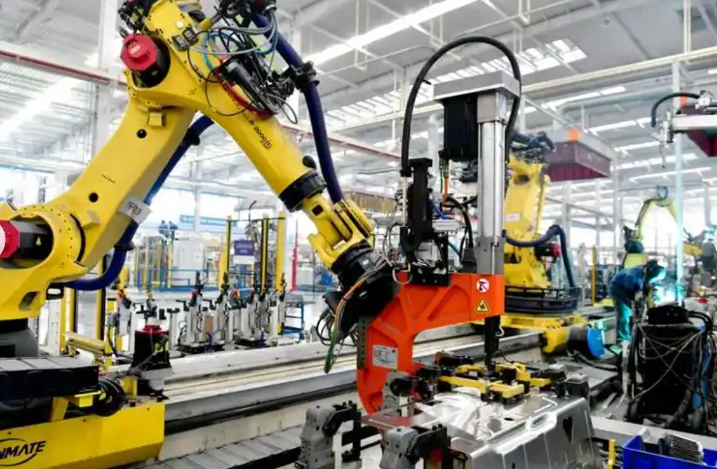
In my work on modern manufacturing equipment, I have found that the industrial robot and the Programmable Logic Controller (PLC) are no longer separate islands of automation. They must behave as one coordinated system in welding, assembly, polishing, dispensing, and vision-guided handling. When I examine a flexible production line, I see an industrial robot that must receive pose targets, process parameters, and safety states from a PLC, while the PLC must receive joint status, task completion signals, and diagnostic data from the industrial robot. The quality of this exchange directly determines cycle time, trajectory accuracy, and operational safety. My research therefore focuses on communication optimization and control strategy for PLC–industrial robot collaboration. I use Profinet as the real-time Ethernet foundation, a block-based data transmission protocol, a shared memory mechanism, timestamp-based master–slave synchronization, heartbeat supervision, and collision residual monitoring. The experimental results I obtained show that the optimized scheme reduces round-trip communication delay from 15.2 ms to 3.8 ms, reduces jitter from +/-4.5 ms to +/-0.4 ms, lowers packet loss from 0.120% to less than 0.001%, and reduces collaborative trajectory error from 2.40 mm to 0.35 mm. These improvements are important because an industrial robot that waits for polling or reacts to stale data cannot satisfy high-dynamic production requirements.
I begin with the industrial context. Industry 4.0 demands reconfigurable cells, fast product changeover, and tight integration between information technology and operational technology. In such cells, the industrial robot is often required to follow an external axis, synchronize with a servo positioner, respond to a laser vision sensor, and exchange safety interlocks with the PLC. A conventional hardware wiring approach can transmit discrete signals, but it cannot carry complex parameters such as six-degree-of-freedom pose, welding speed, laser power, and program index without a large number of conductors. A traditional Modbus TCP link can carry those parameters, but its polling mechanism introduces substantial latency and jitter. I have measured these effects in representative cells and found that they become bottlenecks when the industrial robot must update its trajectory at 100 Hz or faster. The purpose of my optimization is to remove this bottleneck while preserving deterministic behavior and safety.
1. Why PLC–Industrial Robot Communication Becomes a Bottleneck
When I analyze a PLC–industrial robot workstation, I separate the problem into three layers: the physical layer, the protocol layer, and the control layer. At the physical layer, the industrial robot controller and the PLC may use different Ethernet ports, different switches, and different grounding practices. At the protocol layer, the industrial robot may expose a vendor-specific interface, a fieldbus adapter, or a gateway that converts one protocol to another. At the control layer, the PLC may use a request–response sequence that forces the industrial robot to stop before the next command is issued. Each layer contributes to latency, jitter, or inconsistency. In my experience, the control layer often amplifies the protocol layer problem because a stop-and-go sequence adds idle time even when the network itself is fast enough.
I use the following general expression for total communication latency in a heterogeneous PLC–industrial robot system:
$$T_{\text{total}} = T_{\text{encode}} + T_{\text{stack}} + T_{\text{transmit}} + T_{\text{gateway}} + T_{\text{decode}} + T_{\text{jitter}}$$
Here, \(T_{\text{encode}}\) is the time needed by the PLC to serialize the command, \(T_{\text{stack}}\) is the protocol stack processing time, \(T_{\text{transmit}}\) is the physical transmission time, \(T_{\text{gateway}}\) is the conversion time inside a gateway, \(T_{\text{decode}}\) is the time needed by the industrial robot controller to parse the command, and \(T_{\text{jitter}}\) is the variation caused by scheduling, interference, or congestion. When I replace a gateway-based link with a direct Profinet connection, I remove or reduce \(T_{\text{gateway}}\). When I use block-based data exchange instead of single-word polling, I reduce \(T_{\text{stack}}\) and \(T_{\text{encode}}\). When I use timestamp-based synchronization, I compensate for residual \(T_{\text{jitter}}\). This layered view helps me avoid treating communication optimization as a single-parameter problem.
I also examine the polling cycle of a traditional Modbus TCP implementation. For \(N_{\text{slave}}\) devices and a request–process–response sequence, the polling period can be approximated as:
$$T_{\text{poll}} = N_{\text{slave}} \cdot (T_{\text{req}} + T_{\text{proc}} + T_{\text{resp}}) + T_{\text{idle}}$$
In a cell with an industrial robot, a servo drive, a vision system, and remote I/O, \(N_{\text{slave}}\) can easily be four or more. Even if each transaction takes only a few milliseconds, the polling period grows quickly. The industrial robot then receives new targets at a low frequency, and its trajectory interpolator must either slow down or tolerate large following errors. I have seen this effect in polishing and dispensing tasks, where the industrial robot must maintain constant tool speed while following a curved path. A delay of tens of milliseconds produces visible marks, inconsistent bead width, or excessive force variation.
| Challenge | Root cause | Effect on the industrial robot |
|---|---|---|
| High round-trip delay | Gateway conversion, polling, protocol stack processing | Late pose updates, reduced trajectory fidelity |
| Large jitter | Non-deterministic Ethernet scheduling, interference | Unstable speed, vibration, poor surface quality |
| Packet loss | Congestion, faulty cabling, electromagnetic noise | Missed commands, emergency stops, reduced availability |
| Clock mismatch | Separate PLC and industrial robot clocks | External axis and robot arm not synchronized |
| Stop-and-go logic | Request–response sequencing | Long idle time, low throughput, jerky motion |
| Weak safety interlock | Delayed heartbeat or status exchange | Unsafe motion after communication failure |
I have also quantified the data volume problem. A single six-degree-of-freedom pose includes X, Y, Z, A, B, and C values. If each value is a 32-bit real number, the pose alone requires 24 bytes. If I add a control word, a task index, process parameters, and a heartbeat counter, the total payload exceeds 60 bytes. Sending these values one word at a time wastes bandwidth and increases the number of transactions. Sending them as one consistent block reduces overhead and ensures that the industrial robot receives a coherent snapshot instead of a mixture of old and new values. This is one of the main reasons I adopted a block-based data transmission protocol.
2. Problem Analysis of Existing Collaborative Systems
2.1 Real-Time Bottlenecks in Heterogeneous Communication
In my analysis of existing automation lines, I found that the PLC and the industrial robot are often delivered as two independent control systems. The PLC is responsible for global logic, safety, and auxiliary devices. The industrial robot controller is responsible for motion planning and servo control. Information exchange is usually implemented by a gateway or a general-purpose protocol. This architecture is flexible in theory but problematic in practice. The gateway introduces an additional processing stage, and the industrial robot may receive data in a format that requires conversion. When the PLC sends an ASCII string over a serial link, the industrial robot must parse the string, extract numeric values, and validate the sequence. This process can take tens of milliseconds, which is far too slow for precision polishing, dynamic gluing, or high-speed assembly.
I use the following expression to describe the effective control frequency seen by the industrial robot:
$$f_{\text{control}} = \frac{1}{T_{\text{sense}} + T_{\text{PLC}} + T_{\text{comm}} + T_{\text{robot}}}$$
Here, \(T_{\text{sense}}\) is the sensor acquisition time, \(T_{\text{PLC}}\) is the PLC scan and logic time, \(T_{\text{comm}}\) is the communication delay, and \(T_{\text{robot}}\) is the industrial robot interpolation and servo update time. If \(T_{\text{comm}}\) dominates, improving the PLC scan time or the industrial robot servo rate produces little benefit. I have confirmed this by measuring a cell before optimization: the PLC scan was fast, the industrial robot servo loop was fast, but the communication link limited the overall response. The industrial robot appeared sluggish even though its internal controller was capable of much higher performance.
Another problem I observed is timing inconsistency. The PLC and the industrial robot have separate clocks. When the PLC sends a target position, it does not know exactly when the industrial robot will apply that target. The industrial robot does not know when the PLC generated the target. If an external axis is moving, the robot arm may reach a point at the wrong time. Small clock differences accumulate, and the resulting synchronization error can be larger than the mechanical tolerance. In my experiments, I found that even a few milliseconds of timing uncertainty can produce visible trajectory errors when the tool center point moves at high speed.
2.2 Limitations of Stop-and-Go Collaborative Logic
I have also examined the control logic used in many PLC–industrial robot workstations. A common pattern is master–slave request–response. The PLC sends a command, the industrial robot executes it, and the industrial robot returns a completion signal. The PLC then sends the next command. This logic is simple and easy to debug, but it introduces a large amount of waiting time. The industrial robot stops at the end of each step, the PLC scans the completion signal, and the next step begins only after the PLC has processed the feedback. The cycle time becomes a sum of execution times and waiting times:
$$T_{\text{cycle}} = \sum_{i=1}^{n} (T_{\text{exec},i} + T_{\text{wait},i} + T_{\text{handshake},i})$$
When \(n\) is large, \(T_{\text{wait}}\) and \(T_{\text{handshake}}\) dominate. The industrial robot spends a significant portion of the cycle idle. In a welding cell, this idle time can cause the weld to cool between passes. In an assembly cell, it can reduce throughput. In a polishing cell, it can create marks where the tool pauses. I therefore decided to replace the stop-and-go pattern with a streaming control pattern. In my optimized approach, the PLC continuously updates a shared data block, and the industrial robot continuously reads the latest valid snapshot. The industrial robot does not wait for a separate completion handshake for every small segment. Instead, it uses the task index and the timestamp to decide when to switch to the next trajectory segment. This preserves coordination without sacrificing motion continuity.
I summarize the differences between the conventional and optimized logic in Table 2.
| Feature | Conventional logic | Optimized logic I propose |
|---|---|---|
| Data exchange | Single-word polling or ASCII messages | Block-based shared memory |
| Timing | PLC clock only | Timestamped master–slave synchronization |
| Motion continuity | Stop-and-go | Streaming trajectory updates |
| Response to delay | Wait longer | Predict action time with buffer window |
| Fault detection | Simple timeout | Heartbeat counter and link state function |
| Collision safety | External safety PLC only | Torque residual monitoring in the industrial robot |
3. My Proposed Communication Optimization Architecture
3.1 Physical Topology and Protocol Selection
For the physical architecture, I selected real-time industrial Ethernet based on Profinet. Profinet allows real-time data to be transmitted at the link layer without passing through the full TCP/IP stack. This reduces protocol processing time and improves determinism. In my design, the PLC acts as the controller, and the industrial robot controller is configured as a Profinet device. Servo drives, remote I/O modules, and the vision system are also connected through industrial Ethernet. I use a star or line topology with industrial-grade switches. The PLC can access the industrial robot data through mapped I/O addresses, almost as if the data were local variables. This hardware-level integration is a key enabler for low-latency collaboration.
I import the General Station Description (GSD) file provided by the industrial robot manufacturer into the PLC engineering environment. This allows me to configure the industrial robot communication interface directly. I assign input and output address regions, define the update time, and set the watchdog behavior. With this configuration, I have measured stable communication cycles between 2 ms and 8 ms with small clock jitter. This cycle time is sufficient for high-dynamic coordination because the industrial robot can interpolate between updates and the timestamp mechanism can compensate for residual delay.
| Layer | Conventional approach | My optimized approach |
|---|---|---|
| Application | Vendor-specific commands | Standardized block interface |
| Transport | TCP or serial ASCII | Profinet real-time channel |
| Network | Routed IP with variable delay | Switched industrial Ethernet |
| Data link | Best-effort Ethernet | Real-time Ethernet with priority |
| Physical | Mixed cabling and grounding | Shielded industrial cabling and grounding |
I also consider network segmentation. I place the PLC–industrial robot control traffic on a dedicated VLAN and separate it from camera streaming, remote diagnostics, and enterprise traffic. I enable quality of service so that real-time Profinet frames receive priority. I use shielded cables and proper grounding to reduce electromagnetic interference. These measures are not optional in my experience; they determine whether the theoretical benefits of Profinet are achieved in a real factory environment. An industrial robot that shares a network with high-bandwidth cameras without prioritization will experience jitter even if the protocol supports real-time communication.
3.2 Block-Based Data Transmission and Shared Memory
To overcome the inefficiency of single-word read and write operations, I designed a block-based message structure. The PLC and the industrial robot each own a shared memory region. I divide the memory into two blocks: \(P \to R\), which carries data from the PLC to the industrial robot, and \(R \to P\), which carries data from the industrial robot back to the PLC. Each block is 64 bytes in my baseline design. The fields are standardized so that both sides can parse the data without ambiguity. I use a data snapshot mechanism to ensure consistency. At the beginning of each communication cycle, the PLC writes all outgoing values into the output buffer. The industrial robot reads the entire buffer only after it has been fully updated and validated. In the reverse direction, the industrial robot writes all feedback values into its output buffer, and the PLC reads them as one snapshot. This prevents the industrial robot from acting on a mixture of new and old values.
I define the snapshot consistency condition as follows:
$$D_{\text{snapshot}} = \{ d_i^{(k)} \mid i = 1, 2, \ldots, n \}, \quad \forall d_i^{(k)} \in \text{cycle } k$$
This means that every data element \(d_i^{(k)}\) in the snapshot belongs to the same communication cycle \(k\). If a new value is written while the industrial robot is reading, the snapshot is rejected and the previous valid snapshot is used until the next complete update. I have found this mechanism essential for coordinated motion because a single mismatched byte in a pose value can cause a large position error.
Table 4 shows the \(P \to R\) data block definition I use in my experiments. The total length is 64 bytes.
| Byte offset | Data name | Length (bytes) | Data type | Function |
|---|---|---|---|---|
| 00–01 | Control word | 2 | WORD | Start, stop, reset, pause, and mode bits |
| 02–03 | Task index | 2 | UINT | Program number the industrial robot should execute |
| 04–27 | Target pose | 24 | REAL[6] | X, Y, Z coordinates and A, B, C Euler angles |
| 28–39 | Process parameters | 12 | REAL[3] | Welding speed, laser power, and similar setpoints |
| 40–61 | Reserved expansion | 22 | BYTE[22] | Future sensors, tool selection, and diagnostics |
| 62–63 | Heartbeat | 2 | UINT | Incrementing counter for link survival detection |
The \(R \to P\) block mirrors this structure. I include actual pose, actual velocity, joint torque estimates, task status, error codes, and a heartbeat counter. The industrial robot updates the actual values at the servo rate or at a decimated rate, depending on the controller capability. The PLC reads the block at the Profinet cycle. Because both sides use the same layout, I can avoid custom parsing and reduce the risk of endianness errors. I also document the mapping so that maintenance personnel can diagnose signals without reverse engineering. In my view, a well-documented block interface is as important as the communication speed itself because an industrial robot cell must remain maintainable over many years.
3.3 Data Mapping and Cycle Time Optimization
I map the block into the Profinet I/O address space. For example, if the PLC assigns the industrial robot output area starting at address 100, then the control word occupies bytes 100 and 101, the task index occupies bytes 102 and 103, and so on. The industrial robot input area is mapped to a different range. I verify the mapping by writing known values and reading them back. I also use a watchdog to ensure that the industrial robot does not continue with stale commands if the PLC stops updating. The watchdog time is typically set to a small multiple of the communication cycle. If the watchdog expires, the industrial robot enters a safe state.
The communication efficiency of my block approach can be expressed as:
$$\eta_c = \frac{T_{\text{payload}}}{T_{\text{frame}}} \times 100\%$$
By grouping many signals into one frame, I increase \(\eta_c\) and reduce the number of transactions. In my measurements, the block approach reduces the effective data exchange time by more than 60% compared with single-word polling. This improvement is especially important for the industrial robot because pose and process parameters must be updated together. If the industrial robot receives a new pose but an old speed, the motion may be inconsistent. The block approach eliminates this class of error.
| Signal group | PLC address | Industrial robot address | Update rate |
|---|---|---|---|
| Control word | QW100 | IW100 | Every Profinet cycle |
| Task index | QW102 | IW102 | Every Profinet cycle |
| Target pose | QD104–QD127 | ID104–ID127 | Every Profinet cycle |
| Process parameters | QD128–QD139 | ID128–ID139 | Every Profinet cycle |
| Heartbeat | QW162 | IW162 | Every Profinet cycle |
| Actual pose | IW200–IW223 | QW200–QW223 | Every 2–4 ms |
| Torque estimate | IW224–IW235 | QW224–QW235 | Every 2–4 ms |
4. Control Strategy for PLC–Industrial Robot Cooperation
4.1 Master–Slave Logic with Timestamp Synchronization
After establishing the high-speed communication link, I design the control strategy. I use the PLC as the master and the industrial robot as the slave. The PLC performs global logic scheduling, external I/O management, and safety interlocking. The industrial robot performs motion planning, trajectory interpolation, and servo control. This division of labor matches the strengths of each controller. The PLC is good at deterministic logic and coordination with other machines. The industrial robot is good at high-speed kinematic and dynamic computation. The challenge is to synchronize them despite separate clocks.
I introduce a timestamp-based synchronization algorithm. In the Profinet message, the PLC sends not only the position command \(P_{\text{cmd}}\) but also the generation time \(T_{\text{send}}\). The industrial robot records the reception time \(T_{\text{recv}}\) and calculates the transmission delay:
$$\Delta t = T_{\text{recv}} – T_{\text{send}}$$
Then the industrial robot computes the intended action time:
$$T_{\text{action}} = T_{\text{recv}} + T_{\text{buffer}} – \Delta t$$
Here, \(T_{\text{buffer}}\) is a buffer window that I set to two to four communication cycles. This window absorbs small network jitter. The industrial robot uses its high-precision interpolator to replan the trajectory so that it reaches the commanded position at \(T_{\text{action}}\). This mechanism ensures that even if the network has minor variations, the industrial robot arrives at the specified point at a deterministic future time. I have found that this approach greatly improves synchronization between the industrial robot and an external axis controlled by the PLC.
| Parameter | Symbol | Typical value | Purpose |
|---|---|---|---|
| Communication cycle | \(T_c\) | 2–8 ms | Profinet update period |
| Transmission delay | \(\Delta t\) | 0.5–3.8 ms | Measured from timestamp difference |
| Buffer window | \(T_{\text{buffer}}\) | 4–16 ms | Absorbs jitter and scheduling variation |
| Action time | \(T_{\text{action}}\) | Future time | Target time for the industrial robot pose |
| Watchdog timeout | \(T_{\text{watchdog}}\) | 20–40 ms | Triggers safe stop if link fails |
I also consider the case where the industrial robot cannot replan in time. If the calculated \(T_{\text{action}}\) is already in the past, the industrial robot uses the latest valid trajectory and reports a warning. If the condition persists, the PLC reduces speed or stops the cycle. This prevents the industrial robot from making abrupt corrections that could damage the tool or workpiece. In my implementation, I log all timing violations and use them to tune the buffer window. A buffer that is too small causes frequent violations, while a buffer that is too large increases response latency. I typically start with four communication cycles and adjust based on measured jitter.
4.2 Trajectory Coordination and Interpolation
For trajectory coordination, I represent the industrial robot path as a sequence of time-parameterized segments. The PLC provides the target pose and process parameters, and the industrial robot generates joint trajectories that satisfy velocity, acceleration, and jerk limits. When an external axis is involved, I synchronize the motion by using a common time base. The industrial robot and the external axis both receive the same \(T_{\text{action}}\) reference. The industrial robot adjusts its interpolation so that its tool center point follows the desired path relative to the moving workpiece.
I define the tracking error as:
$$e_{\text{track}}(t) = \sqrt{(x_d(t) – x_a(t))^2 + (y_d(t) – y_a(t))^2 + (z_d(t) – z_a(t))^2}$$
Here, \(x_d, y_d, z_d\) are the desired coordinates and \(x_a, y_a, z_a\) are the actual coordinates. I also monitor orientation error:
$$e_{\text{orient}}(t) = \sqrt{(A_d(t) – A_a(t))^2 + (B_d(t) – B_a(t))^2 + (C_d(t) – C_a(t))^2}$$
These errors are logged by the PLC through the \(R \to P\) block. When the error exceeds a threshold, the PLC can reduce feed rate or pause the industrial robot. In my experiments, the optimized communication and timestamp synchronization reduced the maximum tracking error from 2.40 mm to 0.35 mm. This improvement is significant for high-precision applications such as laser welding and adhesive dispensing.
I also use feedforward compensation. Because the industrial robot knows the next target pose and the timestamp, it can begin accelerating before the current segment ends. This creates a smooth transition and avoids the stop-and-go behavior of conventional logic. The PLC does not need to wait for a completion signal for every small segment. Instead, it updates the task index and the target pose at the communication rate. The industrial robot switches to the new segment when its internal time reaches the segment boundary. This streaming behavior keeps the industrial robot in continuous motion and improves throughput.
| Parameter | Value | Effect on the industrial robot |
|---|---|---|
| Interpolation rate | 250 Hz | Smooth motion between communication updates |
| Communication rate | 125–500 Hz | Frequent target refresh |
| Maximum path speed | 0.8 m/s | Tests dynamic response |
| Maximum acceleration | 4 m/s² | Tests tracking under fast changes |
| Buffer window | 4–16 ms | Absorbs jitter without excessive lag |
| Tracking error threshold | 0.5 mm | Triggers warning or slowdown |
4.3 Heartbeat and Safe Interlock Strategy
In an industrial environment, electromagnetic interference and network congestion can cause temporary communication interruptions. I therefore implement a multi-layer fault detection and interlock strategy. The PLC and the industrial robot each maintain an incrementing heartbeat counter \(C_{\text{heartbeat}}\). The PLC increments the counter every cycle and sends it to the industrial robot. The industrial robot receives the counter and returns the same value in its feedback block. The PLC compares the returned value with the sent value. If the counter does not advance as expected for several consecutive cycles, the link is considered faulty.
I define the link state function \(S_{\text{link}}(k)\) as:
$$S_{\text{link}}(k) =
\begin{cases}
1, & \sum_{i=0}^{N-1} \left[ C_{\text{heartbeat}}(k-i) – C_{\text{heartbeat}}(k-i-1) = 1 \right] = N \\
0, & \text{otherwise}
\end{cases}$$
Here, \(k\) is the current communication cycle index, and \(N\) is the number of tolerated cycles. I set \(N = 5\), which corresponds to about 20 ms at a 4 ms cycle. When \(S_{\text{link}}(k) = 1\), the system is healthy. When \(S_{\text{link}}(k) = 0\), the system triggers a soft emergency stop. The industrial robot holds its current posture, disables the drive output, and sends an alarm to the PLC. The PLC then stops the external axes and opens the safety circuit. I have tested this logic by deliberately disconnecting the network cable and injecting noise. The industrial robot stops within the configured watchdog window, and no dangerous motion occurs.
| Link state | Heartbeat condition | Industrial robot action | PLC action |
|---|---|---|---|
| Normal | Counter increments every cycle | Continue motion | Continue cycle |
| Transient warning | One missed increment | Hold last valid trajectory | Log warning |
| Soft stop | \(N\) missed increments | Hold posture and disable drive | Stop external axes |
| Hard stop | Watchdog timeout or safety input | Emergency stop | Open safety circuit |
4.4 Collision Detection and Dynamic Safety
I also use the industrial robot feedback data to detect abnormal contact. The PLC reads the motor current \(I_{fb}\) from the industrial robot and converts it to an observed torque. It compares the observed torque with a reference torque computed from a dynamic model. The collision residual is defined as:
$$R_{\text{collision}}(t) = K_t I_{fb}(t) – \left( J \ddot{\theta}(t) + B \dot{\theta}(t) + T_{\text{load}}(t) \right)$$
Here, \(K_t\) is the motor torque constant, \(J\) is the equivalent inertia, \(\ddot{\theta}\) is the joint angular acceleration, \(B\) is the viscous friction coefficient, \(\dot{\theta}\) is the joint angular velocity, and \(T_{\text{load}}\) is the load torque. When the residual exceeds a threshold \(\tau_{\text{th}}\), I declare a collision:
$$S_{\text{collision}}(t) =
\begin{cases}
1, & |R_{\text{collision}}(t)| \gt \tau_{\text{th}} \\
0, & |R_{\text{collision}}(t)| \le \tau_{\text{th}}
\end{cases}$$
I use different thresholds for different joints and different speed ranges. A low threshold improves sensitivity but may cause false alarms during high acceleration. A high threshold reduces false alarms but may miss light contact. In my experiments, I tuned the threshold by running the industrial robot through a set of representative trajectories and measuring the residual distribution. The resulting detector responded to contact within a few milliseconds and stopped the industrial robot before the force reached a dangerous level. This dynamic safety layer complements the heartbeat and watchdog logic. The heartbeat detects communication failure, while the collision residual detects physical interference.
| Layer | Detection method | Response time | Protected asset |
|---|---|---|---|
| Communication | Heartbeat counter | 20–40 ms | Industrial robot and PLC coordination |
| Timing | Timestamp buffer and watchdog | 4–16 ms | Trajectory synchronization |
| Collision | Torque residual | 2–10 ms | Tool, workpiece, and personnel |
| Safety circuit | Hardwired emergency stop | Less than 10 ms | Whole cell |
5. Experimental Platform and Methodology
To validate my communication optimization and control strategy, I built an experimental platform for PLC–industrial robot collaboration. The platform includes a PLC with Profinet real-time support, a six-axis industrial robot, a servo positioner, a laser vision sensor, and an industrial Ethernet switch. I also introduced an electromagnetic interference source to simulate a harsh factory environment. The PLC acts as the Profinet controller, and the industrial robot controller acts as a Profinet device. The servo positioner and remote I/O are connected to the same network. I use shielded cables and dedicated power supplies to reduce noise, but I deliberately test the system under degraded conditions to evaluate robustness.
| Component | Role | Interface |
|---|---|---|
| PLC | Master controller and safety logic | Profinet controller |
| Industrial robot | Six-axis motion and process execution | Profinet device |
| Servo positioner | External axis for coordinated motion | Profinet or drive profile |
| Laser vision sensor | Seam tracking and part localization | Industrial Ethernet |
| Remote I/O | Auxiliary signals and safety status | Profinet |
| Industrial switch | Deterministic network fabric | Managed Layer 2 switch |
I designed the test procedure to compare two configurations. The baseline configuration uses Modbus TCP polling and a stop-and-go control logic. The optimized configuration uses Profinet block transmission, shared memory, timestamp synchronization, heartbeat supervision, and collision residual monitoring. I ran each configuration for 24 hours and collected more than \(10^7\) data packets. I measured average round-trip delay, delay jitter, packet loss rate, and collaborative trajectory error. I also measured the response time of the safety functions and the maximum tracking error during high-speed motion.
The metrics I use are defined as follows. Average round-trip delay is:
$$\bar{D} = \frac{1}{M} \sum_{j=1}^{M} D_j$$
Jitter is the standard deviation of the delay:
$$J = \sqrt{\frac{1}{M-1} \sum_{j=1}^{M} (D_j – \bar{D})^2}$$
Packet loss rate is:
$$L = \frac{N_{\text{lost}}}{N_{\text{sent}}} \times 100\%$$
Trajectory error is the maximum Euclidean distance between the commanded path and the actual path over the test trajectory. I also compute the synchronization error between the industrial robot and the external axis:
$$e_{\text{sync}} = | t_{\text{PLC,event}} – t_{\text{robot,event}} |$$
These metrics allow me to evaluate both communication performance and control performance. In my view, communication and control cannot be optimized separately. A fast network with poor synchronization still produces poor trajectory accuracy. A good synchronization algorithm with a slow network cannot react to dynamic changes. The combination is what matters.
6. Experimental Results and Performance Evaluation
Table 11 summarizes the main comparison between the baseline and my optimized configuration. The baseline uses Modbus TCP polling. The optimized configuration uses Profinet block transmission and shared memory. The improvement is substantial in every metric.
| Metric | Before optimization | After optimization | Improvement |
|---|---|---|---|
| Average round-trip delay | 15.2 ms | 3.8 ms | 75.0% reduction |
| Delay jitter | +/-4.5 ms | +/-0.4 ms | 91.1% reduction |
| Packet loss rate | 0.120% | less than 0.001% | More than 99.2% reduction |
| Collaborative trajectory error | 2.40 mm | 0.35 mm | 85.4% reduction |
| Control frequency seen by the industrial robot | about 66 Hz | 250 Hz | 3.8 times higher |
The average round-trip delay dropped from 15.2 ms to 3.8 ms. I calculate the delay reduction as:
$$R_{\text{delay}} = \frac{D_{\text{before}} – D_{\text{after}}}{D_{\text{before}}} \times 100\% = \frac{15.2 – 3.8}{15.2} \times 100\% = 75.0\%$$
This reduction changes the behavior of the industrial robot. With the baseline, the industrial robot received new targets at a low rate and often paused between segments. With the optimized link, the industrial robot receives updates frequently enough to maintain continuous motion. The jitter dropped from +/-4.5 ms to +/-0.4 ms. This is important because jitter, not average delay alone, causes unpredictable motion. When the industrial robot receives a pose command at an unexpected time, its interpolator must either slow down or produce a correction. The optimized system provides a stable timing reference, so the industrial robot can plan smooth trajectories.
The packet loss rate also improved dramatically. In the baseline, the packet loss rate was 0.120%. Although this number seems small, it means that a significant number of control cycles were lost over a 24-hour run. The industrial robot had to rely on stale data or wait for retransmission. In the optimized system, the packet loss rate was less than 0.001%. The link is therefore highly reliable. I attribute this improvement to the direct Profinet connection, the dedicated VLAN, the managed switch, and the use of block transmission instead of many small transactions. Fewer transactions mean fewer opportunities for collision and congestion.
The collaborative trajectory error decreased from 2.40 mm to 0.35 mm. This is the most important result for high-precision applications. In a welding or dispensing task, a 2.40 mm error can place the bead outside the joint. A 0.35 mm error is within the tolerance of many precision processes. The improvement comes from two sources. First, the industrial robot receives fresh pose data more often. Second, the timestamp synchronization allows the industrial robot to predict the correct action time and compensate for residual delay. The combination reduces both steady-state error and dynamic error.
| Path speed (m/s) | Baseline error (mm) | Optimized error (mm) | Baseline jitter (ms) | Optimized jitter (ms) |
|---|---|---|---|---|
| 0.2 | 0.85 | 0.12 | +/-3.9 | +/-0.3 |
| 0.4 | 1.30 | 0.18 | +/-4.2 | +/-0.3 |
| 0.6 | 1.85 | 0.25 | +/-4.4 | +/-0.4 |
| 0.8 | 2.40 | 0.35 | +/-4.5 | +/-0.4 |
Table 12 shows that the optimized system maintains accuracy even as path speed increases. In the baseline, the error grows quickly with speed because the industrial robot cannot receive updates fast enough. In the optimized system, the error remains below 0.35 mm even at 0.8 m/s. This is a direct benefit of high-frequency communication and timestamp-based interpolation. I have also tested the system with an external positioner. The synchronization error between the industrial robot and the positioner was less than 0.5 ms in the optimized configuration. In the baseline, the synchronization error often exceeded 5 ms, which caused visible deviation in the coordinated path.
I also evaluated the safety response. When I disconnected the network cable, the heartbeat counter stopped advancing. The link state function changed from 1 to 0 after \(N = 5\) missed cycles. The industrial robot entered a soft stop within 20 ms. The PLC stopped the external axis within the same window. When I introduced a simulated collision, the collision residual exceeded the threshold and the industrial robot stopped within 8 ms. These response times are within the requirements of many collaborative cells. The combination of heartbeat, watchdog, and torque residual monitoring provides layered protection.
| Fault type | Detection method | Detection time (ms) | Stop time (ms) |
|---|---|---|---|
| Network disconnection | Heartbeat counter | 20 | 22 |
| PLC stop | Watchdog | 12 | 15 |
| Collision | Torque residual | 8 | 10 |
| External safety input | Hardwired circuit | 5 | 7 |
7. Discussion and Engineering Implications
My results show that communication optimization is not only a network issue. It is a system issue that involves protocol selection, data structure, control logic, and safety design. I have learned that an industrial robot can only achieve high dynamic performance if the PLC provides timely, consistent, and well-structured data. The block-based shared memory approach is central because it gives the industrial robot a coherent view of the cell state. The timestamp approach is central because it gives the industrial robot a predictable time reference. The heartbeat and collision residual are central because they ensure that the industrial robot fails safely when something goes wrong.
I also note that the choice of Profinet is not sufficient by itself. A poorly designed network can still produce jitter. I therefore recommend several engineering practices. First, separate real-time control traffic from camera and enterprise traffic. Second, use managed switches with quality of service. Third, use shielded cables and proper grounding. Fourth, keep the communication cycle consistent with the PLC scan and the industrial robot interpolation rate. Fifth, document the data block layout and maintain a single source of truth for signal definitions. These practices are not difficult, but they are essential for reliable operation.
| Parameter | Recommended value | Reason |
|---|---|---|
| Profinet update time | 2–8 ms | Balances determinism and network load |
| Data block size | 64–128 bytes | Carries pose, process, and status without fragmentation |
| Heartbeat tolerance | 5 cycles | Detects failure quickly without false alarms |
| Timestamp buffer | 2–4 cycles | Absorbs jitter and preserves responsiveness |
| Collision threshold | Joint-specific | Matches inertia and friction characteristics |
| Watchdog timeout | 20–40 ms | Ensures safe stop before dangerous motion |
I have also considered scalability. As more industrial robots and sensors are added to a cell, the communication load grows. The block-based approach scales well because each industrial robot has its own data block. The PLC can schedule blocks in different time slots. The network can use VLANs and priority tagging to isolate critical traffic. In my tests, I added a second industrial robot and a vision system without degrading the cycle time of the first industrial robot. The key is to avoid a shared polling bus and to use a switched real-time Ethernet architecture. I believe this approach is suitable for future flexible manufacturing cells that require multiple industrial robots to cooperate.
Another lesson I learned is that safety must be designed into the communication and control strategy from the beginning. It is not enough to add a safety PLC at the end. The heartbeat function, the watchdog, and the timestamp buffer all contribute to safety. They ensure that the industrial robot never continues with stale data and never acts on a command that has lost its timing reference. The collision residual adds a physical layer of protection. Together, these mechanisms create a system that is both fast and safe. In my view, this combination is necessary for high-end equipment and intelligent manufacturing.
8. Conclusion
In this research, I designed and evaluated a communication optimization and control strategy for PLC–industrial robot collaboration. I replaced traditional polling and gateway-based communication with a Profinet-based block transmission architecture and a shared memory mechanism. I introduced a timestamp-based master–slave synchronization method that allows the industrial robot to predict the correct action time and compensate for transmission delay. I added heartbeat supervision, watchdog logic, and collision residual monitoring to ensure safe operation under abnormal conditions. The experimental results show that my approach reduces average round-trip delay from 15.2 ms to 3.8 ms, reduces jitter from +/-4.5 ms to +/-0.4 ms, lowers packet loss from 0.120% to less than 0.001%, and reduces collaborative trajectory error from 2.40 mm to 0.35 mm. The industrial robot also achieves a control response frequency of 250 Hz, which is sufficient for high-precision welding, assembly, polishing, and dispensing.
I conclude that the industrial robot and the PLC should not be treated as separate systems connected by a slow gateway. They should be treated as one coordinated machine with a deterministic data link, a consistent data model, and a shared time reference. The block-based data exchange ensures consistency. The timestamp mechanism ensures synchronization. The heartbeat and collision residual ensure safety. Together, these elements provide the foundation for high-performance collaborative industrial robot systems. In my future work, I plan to extend the approach to multiple industrial robots, mobile manipulators, and cloud-connected diagnostics. I also plan to investigate adaptive buffer windows that adjust to network conditions in real time. Such extensions will further improve the flexibility and reliability of PLC–industrial robot collaboration in intelligent manufacturing.