
In recent years, the locomotion mechanisms inherent in自然界动物 have increasingly captivated researchers in robotics, prompting deep investigations into their implementation in mechanical systems. As a bionic robot enthusiast, I have focused on hexapod designs that mimic creatures like spiders, crabs, and geckos to enhance adaptability and mobility over unstructured terrains. These bionic robots typically feature legs with three joints: a root joint, a hip joint, and a knee joint, allowing versatile leg postures. When employing a tripod gait, the hexapod bionic robot transforms into a 3-UR parallel mechanism during the support phase, where three legs work in concert to propel the body forward. This parallel configuration is crucial for stability and speed, making it a prime subject for kinematic analysis. In this article, I delve into the parallel kinematics of such a hexapod bionic robot, utilizing screw theory and product-of-exponentials for forward kinematics and elimination methods for inverse kinematics. My goal is to provide a comprehensive model that can serve as a foundation for dynamic analysis and control of bionic robots, with an emphasis on clarity through formulas and tables.
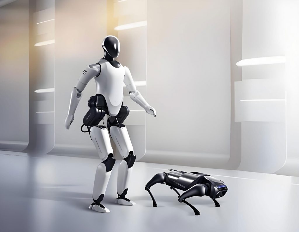
The tripod gait is a common choice for hexapod bionic robots due to its high stability and rapid motion. In this gait, legs are grouped into two sets: one set consists of legs at opposite ends on one side and the middle leg on the other side, while the other set comprises the remaining legs. During locomotion, these sets alternate between swing and support phases. When three legs are in support, they form a 3-UR parallel mechanism with the body, enabling simultaneous摆动和移动. This design not only improves forward velocity but also ensures robustness, which is essential for bionic robots navigating complex environments. To simplify the analysis, I consider the body as an equilateral triangle platform, with coordinate frames attached to both the upper and lower platforms. The upper platform, representing the robot body, is treated as fixed, while the lower platform, formed by the supporting feet, is considered moving. This relative perspective allows us to compute the pose of the lower platform relative to the upper one and then transform it to obtain the body’s pose in the inertial frame.
In bionic robot design, each leg is modeled as a serial chain with three revolute joints. For leg 1, which I analyze in detail, the root joint rotates about the z-axis, the hip joint about the y-axis (negative direction), and the knee joint also about the y-axis (negative direction). The initial configuration has link 2 and link 3 aligned horizontally along the x-axis, with link 4 oriented along the y-axis. The lengths are denoted as $l_2$ and $l_3$ for links 2 and 3, respectively. Using screw theory, I define the joint screw axes for leg 1. For joint $i$ (where $i = 1, 2, 3$), the screw axis is represented as $\xi_i = [v_i, w_i]^T$, where $w_i$ is the unit direction vector of the axis, and $v_i = -w_i \times q_i$, with $q_i$ being a point on the axis. Specifically:
- For joint 1: $w_1 = [0, 0, 1]^T$, $q_1 = [0, 0, 0]^T$, so $v_1 = [0, 0, 0]^T$.
- For joint 2: $w_2 = [0, -1, 0]^T$, $q_2 = [0, 0, 0]^T$, so $v_2 = [0, 0, 0]^T$.
- For joint 3: $w_3 = [0, -1, 0]^T$, $q_3 = [l_2, 0, 0]^T$, so $v_3 = [0, 0, l_2]^T$.
The forward kinematics for leg 1, using the product-of-exponentials formula, is given by:
$$ g(\theta) = e^{\hat{\xi}_1 \theta_1} e^{\hat{\xi}_2 \theta_2} e^{\hat{\xi}_3 \theta_3} g(0) $$
where $g(0)$ is the initial pose of the foot tip relative to the base frame of leg 1. In matrix form, $g(0)$ is:
$$ g(0) = \begin{bmatrix} 1 & 0 & 0 & l_2 + l_3 \\ 0 & 1 & 0 & 0 \\ 0 & 0 & 1 & 0 \\ 0 & 0 & 0 & 1 \end{bmatrix} $$
After computing the exponentials, the foot tip pose relative to the upper platform frame (attached to the body) for leg 1 is derived as $g_1(\theta)$. The position vector $p_1$ of the foot tip is extracted from this matrix. Similar derivations apply to legs 3 and 5, which are symmetrically positioned. For a bionic robot with an equilateral triangular body of side length $l_{\text{upper}}$, the coordinates of leg connection points in the upper platform frame are predefined. After algebraic manipulations, the foot tip positions for legs 1, 3, and 5 are expressed as functions of joint angles $\theta_i$:
$$ p_1 = \begin{bmatrix} l_2 c_1 c_2 + l_3 c_1 c_{23} + \frac{\sqrt{3}}{3} l_{\text{upper}} \\ l_2 s_1 c_2 + l_3 s_1 c_{23} \\ -l_2 s_2 – l_3 s_{23} \end{bmatrix}, \quad p_3 = \begin{bmatrix} -\frac{l_2}{2} c_1 c_2 – \frac{l_3}{2} c_1 c_{23} + \frac{\sqrt{3}}{6} l_{\text{upper}} \\ \frac{\sqrt{3}}{2} l_2 c_1 c_2 + \frac{\sqrt{3}}{2} l_3 c_1 c_{23} + \frac{l_{\text{upper}}}{2} \\ -l_2 s_2 – l_3 s_{23} \end{bmatrix}, \quad p_5 = \begin{bmatrix} -\frac{l_2}{2} c_1 c_2 – \frac{l_3}{2} c_1 c_{23} – \frac{\sqrt{3}}{6} l_{\text{upper}} \\ -\frac{\sqrt{3}}{2} l_2 c_1 c_2 – \frac{\sqrt{3}}{2} l_3 c_1 c_{23} + \frac{l_{\text{upper}}}{2} \\ -l_2 s_2 – l_3 s_{23} \end{bmatrix} $$
where $c_i = \cos(\theta_i)$, $s_i = \sin(\theta_i)$, $c_{ij} = \cos(\theta_i + \theta_j)$, and $s_{ij} = \sin(\theta_i + \theta_j)$. These positions are crucial for determining the lower platform’s pose. The lower platform frame origin is the centroid of the triangle formed by $p_1$, $p_3$, and $p_5$. Using geometry, the pose matrix $g_{\text{lower}}$ of the lower platform relative to the upper platform is computed. By applying the principle of relative motion, the body’s pose matrix $g_{\text{body}}$ in the inertial frame (attached to the lower platform) is obtained as the inverse of $g_{\text{lower}}$.
To facilitate understanding, I summarize the parameters and variables in Table 1, which highlights the key components of this bionic robot system.
| Symbol | Description | Value/Units |
|---|---|---|
| $l_{\text{upper}}$ | Side length of the equilateral triangular body | 20 cm (example) |
| $l_2$ | Length of link 2 (thigh) | 20 cm |
| $l_3$ | Length of link 3 (shank) | 15 cm |
| $\theta_1, \theta_2, \theta_3$ | Joint angles for root, hip, knee | Radians |
| $p_i$ | Foot tip position of leg $i$ in upper frame | Cartesian coordinates (cm) |
| $g_{\text{body}}$ | Body pose matrix in inertial frame | 4×4 homogeneous matrix |
The inverse kinematics problem for this bionic robot involves determining the joint angles given the body’s pose $g_{\text{body}}$. By exploiting the relative motion principle, we first compute $g_{\text{lower}}$ from $g_{\text{body}}$. Then, the foot tip positions $p_1$, $p_3$, and $p_5$ are derived from $g_{\text{lower}}$ using geometric relationships. For instance, from $p_1 = [p_x, p_y, p_z]^T$, we can solve for $\theta_1$, $\theta_2$, and $\theta_3$. Using trigonometric identities and elimination methods, I derive closed-form inverse solutions. For leg 1, the equations are:
$$ \begin{aligned} p_x &= l_2 c_1 c_2 + l_3 c_1 c_{23} + \frac{\sqrt{3}}{3} l_{\text{upper}} \\ p_y &= l_2 s_1 c_2 + l_3 s_1 c_{23} \\ p_z &= -l_2 s_2 – l_3 s_{23} \end{aligned} $$
By manipulating these equations, we obtain:
$$ \theta_1 = \arctan\left(\frac{p_y}{p_x – \frac{\sqrt{3}}{3} l_{\text{upper}}}\right) $$
Then, let $A = p_x – \frac{\sqrt{3}}{3} l_{\text{upper}}$ and $B = p_y$. We have:
$$ \sqrt{A^2 + B^2} = l_2 c_2 + l_3 c_{23} $$
Combining with the $p_z$ equation, we solve for $\theta_2$ and $\theta_3$ using algebraic substitutions. The explicit solutions are:
$$ \theta_2 = \arcsin\left(-\frac{p_z (l_2 + l_3 c_3) – l_3 s_3 \sqrt{A^2 + B^2}}{l_2^2 + l_3^2 + 2 l_2 l_3 c_3}\right) $$
and
$$ \theta_3 = \arccos\left(\frac{(A^2 + B^2) + p_z^2 – l_2^2 – l_3^2}{2 l_2 l_3}\right) $$
These formulas provide the inverse kinematics for leg 1. Similar derivations apply to legs 3 and 5, ensuring the bionic robot can achieve desired poses through coordinated joint movements.
To validate the kinematic models, I conduct a numerical example. Assume the following parameters for the bionic robot: $l_{\text{upper}} = 20 \, \text{cm}$, $l_2 = 20 \, \text{cm}$, $l_3 = 15 \, \text{cm}$. The joint angles for legs 1, 3, and 5 are given in Table 2 as inputs for forward kinematics.
| Leg | $\theta_1$ (rad) | $\theta_2$ (rad) | $\theta_3$ (rad) |
|---|---|---|---|
| 1 | $\pi/6$ | $\pi/6$ | $\pi/4$ |
| 3 | $\pi/4$ | $\pi/4$ | $\pi/6$ |
| 5 | $\pi/6$ | $\pi/6$ | $\pi/6$ |
Using the forward kinematics formulas, I compute the foot tip positions $p_1$, $p_3$, and $p_5$ relative to the upper platform frame. For leg 1:
$$ p_1 = \begin{bmatrix} 20 \cos(\pi/6) \cos(\pi/6) + 15 \cos(\pi/6) \cos(\pi/6 + \pi/4) + \frac{\sqrt{3}}{3} \times 20 \\ 20 \sin(\pi/6) \cos(\pi/6) + 15 \sin(\pi/6) \cos(\pi/6 + \pi/4) \\ -20 \sin(\pi/6) – 15 \sin(\pi/6 + \pi/4) \end{bmatrix} $$
After evaluation, $p_1 \approx [29.91, 10.60, 24.49] \, \text{cm}$. Similarly, $p_3 \approx [11.78, 7.55, 22.99] \, \text{cm}$ and $p_5 \approx [9.84, 19.01, 28.63] \, \text{cm}$. The lower platform pose matrix $g_{\text{lower}}$ is computed from these points using centroid and orientation calculations. Then, the body pose matrix $g_{\text{body}}$ is derived as:
$$ g_{\text{body}} = \begin{bmatrix} 0.06165 & -0.9961 & 0.06348 & -25.31 \\ 0.9916 & 0.06838 & 0.1099 & -50.40 \\ 0.1139 & -0.05617 & -0.9919 & -81.20 \\ 0 & 0 & 0 & 1 \end{bmatrix} $$
For inverse kinematics validation, I use this $g_{\text{body}}$ as input. By reversing the process, I compute $g_{\text{lower}}$, extract $p_1$, $p_3$, and $p_5$, and then apply the inverse kinematics formulas to solve for joint angles. The results match the original inputs in Table 2, confirming the consistency of the models. This verification step is critical for ensuring the reliability of bionic robot control systems.
The advantages of using screw theory and product-of-exponentials for this bionic robot are manifold. First, it provides a compact and elegant representation of kinematics, avoiding the complexities of traditional D-H parameters, especially for motions involving multiple axes. Second, the closed-form inverse solutions enable real-time control, which is essential for bionic robots operating in dynamic environments. Moreover, the parallel mechanism analysis enhances our understanding of stability and force distribution during locomotion. To further illustrate, Table 3 compares the kinematic approaches for bionic robots, highlighting the benefits of the proposed method.
| Method | Advantages | Disadvantages | Suitability for Bionic Robots |
|---|---|---|---|
| D-H Parameters | Standardized, widely used | Cumbersome for multi-axis motions, singularities | Moderate |
| Screw Theory | Geometric intuition, compact formulas | Requires understanding of Lie groups | High |
| Product-of-Exponentials | Direct mapping, avoids coordinate ambiguities | Computational complexity for inverse | High |
| Elimination Methods | Yields closed-form solutions | Algebraically intensive | High for parallel mechanisms |
In practical applications, bionic robots like this hexapod can be used for search-and-rescue, exploration, or agricultural tasks. The kinematic models developed here serve as a foundation for trajectory planning and impedance control. For instance, by prescribing a desired body motion, the inverse kinematics computes the required joint angles, which can be fed to actuators. Additionally, the forward kinematics helps in sensor-based feedback for pose estimation. The integration of these models into a control loop is vital for autonomous operation of bionic robots.
To deepen the analysis, I explore the Jacobian matrix for the parallel mechanism. The Jacobian relates the body velocity to joint velocities, which is key for dynamics and control. For leg 1, the body velocity twist $V_b$ is given by $V_b = J_1(\theta) \dot{\theta}_1$, where $J_1$ is the geometric Jacobian derived from screw theory. For a bionic robot with multiple legs, the overall Jacobian for the parallel support phase is assembled by considering the constraints from all supporting legs. This matrix can be used to analyze singularities and manipulability, ensuring the bionic robot avoids configurations where motion becomes uncontrollable.
Another aspect is the workspace analysis of the bionic robot. The reachable positions of the foot tips determine the body’s mobility. Using the forward kinematics, I can plot the workspace volume for different leg configurations. For example, by varying $\theta_1$, $\theta_2$, and $\theta_3$ within limits (e.g., $\theta_i \in [-\pi/2, \pi/2]$ to avoid self-collision), the foot tip positions form a spatial region. The union of these regions for all legs defines the body’s feasible displacements. This analysis is crucial for gait planning, especially when the bionic robot traverses rough terrain.
In terms of performance metrics, bionic robots often prioritize energy efficiency and stability. The kinematic models allow us to compute metrics like stride length and duty factor. For the tripod gait, the stride length per cycle is related to the body pose change. Assuming a periodic motion, the body translates by $\Delta x$ during each support phase. From the forward kinematics, $\Delta x$ can be expressed as a function of joint angle ranges. For instance, if $\theta_1$ varies from $-\pi/6$ to $\pi/6$, $\theta_2$ from $0$ to $\pi/4$, and $\theta_3$ from $-\pi/3$ to $0$, the resulting $\Delta x$ can be optimized for speed or efficiency.
Furthermore, I consider the impact of design parameters on kinematics. For a bionic robot, leg lengths $l_2$ and $l_3$ influence the workspace and force transmission. Using sensitivity analysis, we can study how changes in these parameters affect the foot tip positions. For example, the partial derivatives $\frac{\partial p_x}{\partial l_2}$ and $\frac{\partial p_z}{\partial l_3}$ indicate the sensitivity to manufacturing tolerances. This is important for robust bionic robot design in real-world applications.
The kinematic analysis also extends to different gait patterns. While the tripod gait is emphasized, bionic robots can employ other gaits like wave or ripple for slower, more stable motion. For each gait, the parallel mechanism configuration changes, requiring adapted kinematic models. For example, in a wave gait, only one leg is in swing at a time, resulting in a series of single-leg support phases. The forward and inverse kinematics can be modified accordingly, showcasing the versatility of bionic robots.
To illustrate the computational aspects, I provide algorithms for solving the kinematics. For forward kinematics, the steps are: 1) Initialize parameters, 2) Compute screw exponentials for each joint, 3) Multiply matrices to get foot tip poses, 4) Compute lower platform pose via centroid, 5) Invert to get body pose. For inverse kinematics, the steps are: 1) Input body pose, 2) Compute lower platform pose, 3) Solve for foot tip positions using geometry, 4) Apply inverse formulas for each leg. These algorithms can be implemented in software for simulating bionic robot motion.
In conclusion, the parallel kinematic analysis of a hexapod bionic robot using screw theory and elimination methods provides a robust framework for modeling and control. The forward kinematics offers a clear mapping from joint angles to body pose, while the inverse kinematics yields closed-form solutions for real-time applications. The validation through numerical examples confirms the models’ accuracy. This work lays the groundwork for future research on dynamics, control strategies, and optimization of bionic robots for diverse tasks. As bionic robots continue to evolve, such kinematic insights will be pivotal in achieving lifelike locomotion and enhanced performance in challenging environments.
Finally, I reflect on the broader implications. Bionic robots inspired by nature offer sustainable solutions for automation, and their kinematic analysis is a stepping stone toward more advanced bio-inspired systems. By integrating sensors and adaptive algorithms, these robots can learn and adjust their gaits dynamically, much like their biological counterparts. The journey from kinematic models to fully autonomous bionic robots is an exciting frontier in robotics, promising innovations that blend engineering with biological principles.