
From my perspective, the intelligent machining production line built around industrial robots is not simply a collection of fast machines. It is a tightly synchronized cyber-physical system in which every robot, machine tool, conveyor, sensor, safety device, and management platform must exchange information with deterministic timing. I have found that the programmable logic controller, or PLC, remains the most practical and reliable anchor for this synchronization. When I design or evaluate a line that uses industrial robots, I treat the PLC as the central nervous system: it collects signals, executes logic, coordinates motion, enforces safety, and prepares data for higher-level analytics. The result is a production line that can switch products, adapt to process variation, and continue operating safely even when individual devices behave differently from their nominal models.
In my work, the phrase “PLC technology” means more than a single hardware unit. It includes the CPU, input and output modules, communication interfaces, safety-rated logic, engineering software, diagnostic functions, and the data structures that connect the controller to industrial robots, computer numerical control machines, automated guided vehicles, vision systems, and enterprise software. I use the PLC to turn discrete events into repeatable sequences and to turn analog measurements into actionable decisions. This is especially important in lines based on industrial robots, because industrial robots are flexible but they require precise handshaking with upstream and downstream equipment. Without a PLC, the industrial robots may perform their individual tasks well, yet the line as a whole may suffer from collisions, idle time, inconsistent quality, and unsafe conditions.
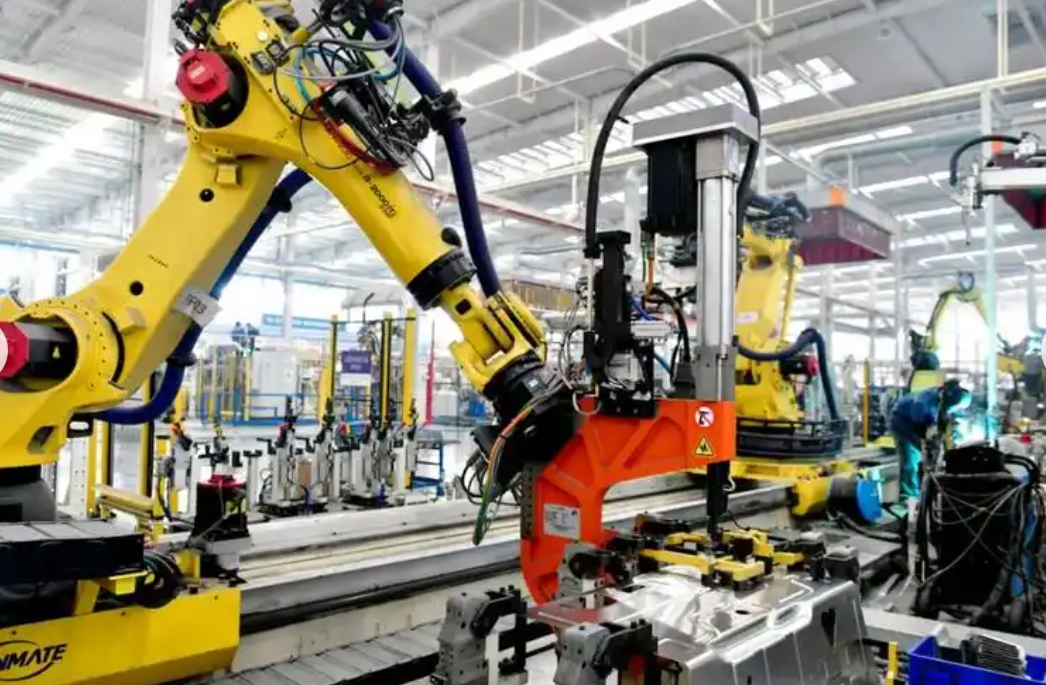
My Understanding of PLC Roles in Industrial Robot Machining Lines
I classify the role of the PLC into four major functions: central control, flexible manufacturing support, intelligent data provisioning, and safety assurance. These functions overlap in practice, but separating them helps me explain why the PLC is still indispensable in an era of edge computing, industrial internet, and artificial intelligence. The industrial robots provide mechanical flexibility, the machine tools provide process capability, and the sensors provide awareness. The PLC provides deterministic coordination. In my experience, deterministic coordination is the difference between a demonstration cell and a production line that can run for multiple shifts with predictable output.
The Central Control Hub
I see the PLC as the central control hub because it receives state signals from every unit and issues commands according to a defined production logic. The input modules read signals from proximity sensors, limit switches, pressure switches, temperature transmitters, force sensors, vision controllers, robot controllers, and safety devices. The CPU executes the user program, which I usually write in ladder diagram, function block diagram, structured text, or a combination of these languages. The output modules then drive contactors, valves, servo enables, robot start signals, conveyor motors, indicator lights, and safety relays. In a line with industrial robots, the PLC often acts as the master sequencer, while each industrial robot controller acts as a subordinate motion controller. The PLC does not usually generate the robot’s joint trajectories, but it tells the industrial robot when to start, which program to run, where to hand off the workpiece, and when to wait.
I use a simple equation to describe the control cycle in my designs:
$$T_{cycle} = T_{input} + T_{scan} + T_{logic} + T_{output} + T_{network}$$
Here, \(T_{input}\) is the time required to read field signals, \(T_{scan}\) is the PLC scan time, \(T_{logic}\) is the time required to execute the control program, \(T_{output}\) is the time required to update outputs, and \(T_{network}\) is the communication delay to industrial robots and other devices. In a well-designed line, the total control cycle must be significantly shorter than the fastest mechanical event that the PLC is expected to detect. When I commission a line, I measure this cycle and compare it with the required response time. If the margin is too small, I increase the CPU performance, optimize the program, or move certain high-speed functions to a dedicated motion controller or safety controller.
| Control Layer | Typical Device | My Primary Concern | Key Signal or Data |
|---|---|---|---|
| Field layer | Sensors, buttons, valves, motor starters | Signal reliability and noise immunity | Discrete states, analog values, diagnostic bits |
| Control layer | PLC CPU, I/O modules, safety PLC | Scan time, logic determinism, redundancy | Sequence states, interlocks, safety outputs |
| Motion layer | Industrial robot controllers, CNC systems, servo drives | Trajectory accuracy and handshaking | Program number, start, busy, complete, fault |
| Supervisory layer | HMI, SCADA, manufacturing execution system | Visibility, traceability, scheduling | Production counts, alarms, recipes, OEE data |
| Enterprise layer | ERP, cloud analytics, digital twin | Long-term optimization and planning | Orders, maintenance history, energy reports |
I also use an interlock equation to express the condition for starting a downstream action:
$$S_{downstream} = S_{upstream} \land S_{robot} \land S_{guard} \land S_{process} \land \neg S_{fault}$$
In this expression, \(S_{upstream}\) indicates that the previous process is complete, \(S_{robot}\) indicates that the industrial robot is in the correct position and ready, \(S_{guard}\) indicates that the safety guard is closed, \(S_{process}\) indicates that the process parameters are within limits, and \(S_{fault}\) indicates that no fault is active. I apply this logic repeatedly in my programs. It prevents the industrial robots from acting before the workpiece is clamped, prevents machine tools from cutting before the industrial robot has released the part, and prevents conveyors from moving before the transfer position is clear.
Flexible Manufacturing Support
I consider flexible manufacturing to be one of the strongest reasons to use a PLC with industrial robots. A line that produces only one product at high volume can sometimes rely on hard-wired logic or dedicated mechanisms. A line that produces multiple products in small batches, however, needs a controller that can change sequences, parameters, and robot programs quickly. The PLC supports this through modular programming. I divide the control program into reusable function blocks: one block for product loading, one for industrial robot handshaking, one for machining, one for inspection, one for unloading, and one for safety recovery. When the product changes, I call a different recipe and adjust a limited set of parameters rather than rewriting the entire program.
I model the changeover time as follows:
$$T_{changeover} = T_{recipe\_load} + T_{robot\_program\_switch} + T_{tool\_adjust} + T_{verification} + T_{ramp\_up}$$
In my experience, PLC-based recipe management can reduce \(T_{recipe\_load}\) and \(T_{robot\_program\_switch}\) to a few seconds or less, while mechanical tool changes and first-piece verification often dominate the total changeover time. This is why I always combine PLC flexibility with quick-change fixtures, preset tooling, and automated parameter verification. The industrial robots can switch programs quickly, but if the fixture is not repeatable, the line will still lose time and quality.
| Product Variant | Robot Program | PLC Recipe Parameters | Fixture or Tool Change | Expected Changeover Time |
|---|---|---|---|---|
| Variant A | Pick and place A | Speed 80%, force limit 120 N, offset 0.0 mm | Fixture A, tool T1 | 4 minutes |
| Variant B | Pick and place B | Speed 65%, force limit 100 N, offset 0.2 mm | Fixture B, tool T2 | 7 minutes |
| Variant C | Pick and place C | Speed 90%, force limit 150 N, offset -0.1 mm | Fixture C, tool T3 | 9 minutes |
| Variant D | Pick and place D | Speed 75%, force limit 110 N, offset 0.1 mm | Fixture D, tool T4 | 6 minutes |
I also use parameter arrays to keep the program organized. For example, I may define an array of robot speed values, an array of machining feed rates, and an array of inspection thresholds. The PLC selects the correct index based on the product code. This approach makes the control logic easier to validate and reduces the risk of an operator editing the wrong parameter. When I work with industrial robots, I insist that the robot program number and the PLC recipe number are cross-checked before the cycle starts. If they do not match, the PLC holds the line and displays an alarm. This simple check prevents many costly mistakes.
Intelligent Decision Data Foundation
I do not view the PLC as only a sequencing device. In modern lines based on industrial robots, the PLC is also a data acquisition and preprocessing node. It reads device status, process values, quality measurements, energy consumption, and alarm codes. It timestamps events, filters noise, converts units, and sends structured data to the supervisory system. I have learned that the quality of high-level analytics depends heavily on the quality of this lower-level data. If the PLC sends raw, uncalibrated, or inconsistent data, then dashboards and artificial intelligence models will produce misleading conclusions.
I use a data normalization formula when I prepare analog values for upper-level systems:
$$x_{norm} = \frac{x_{raw} – x_{min}}{x_{max} – x_{min}}$$
For process variables such as cutting force, temperature, and position error, I also calculate deviation from the target:
$$e = x_{measured} – x_{target}$$
When the absolute deviation exceeds a threshold, the PLC can trigger an alarm, adjust a parameter, or request an inspection. In my architecture, the PLC performs fast deterministic decisions at the edge, while the supervisory system performs slower, more complex optimization. This division of labor is important because industrial robots and machine tools cannot wait for a cloud response before every movement. The PLC must handle immediate interlocks and safety logic locally. The cloud or edge server can analyze trends, predict maintenance, and optimize schedules over longer horizons.
| Data Category | Example Signal | PLC Processing | Upper-Level Use |
|---|---|---|---|
| Device state | Robot auto mode, machine running, conveyor ready | Boolean logic, state machine | OEE calculation, downtime analysis |
| Process value | Cutting force, spindle speed, feed rate, temperature | Scaling, filtering, limit checking | Adaptive control, quality correlation |
| Quality value | Vision pass or fail, dimensional deviation, surface defect count | Pass/fail decision, data tagging | Traceability, statistical process control |
| Energy value | Power draw, air consumption, coolant flow | Accumulation, averaging, peak detection | Energy management, sustainability reporting |
| Maintenance value | Cycle count, motor current, vibration, fault code | Threshold comparison, counter | Predictive maintenance, spare parts planning |
Safety Assurance Barrier
In my designs, safety is never an afterthought. I treat the safety PLC or safety-rated PLC as a separate but coordinated layer. It reads emergency stop buttons, safety light curtains, door switches, two-hand controls, enabling devices, and overload sensors. When a safety function is triggered, the safety PLC must bring the industrial robots and machining equipment to a safe state within a defined time. The standard PLC may continue to manage non-safety functions such as diagnostics and operator messages, but it must not be relied upon for safety-critical actions unless it is designed and certified for that purpose.
I use the following relationship to verify stopping performance:
$$d_{safe} = v_{human} \times (t_{react} + t_{stop}) + d_{margin}$$
Here, \(d_{safe}\) is the minimum safe distance, \(v_{human}\) is the approach speed of a person, \(t_{react}\) is the reaction time, \(t_{stop}\) is the stopping time of the industrial robot or machine, and \(d_{margin}\) is an additional safety margin. I also check the safety response time:
$$T_{safe} = T_{detect} + T_{safety\_PLC} + T_{actuator}$$
If \(T_{safe}\) is too long, I reduce it by selecting faster sensors, using a safety PLC with shorter response time, improving the actuator circuit, or installing physical guards that prevent access before the hazard can be reached. In my experience, the safety PLC must be independent enough to remain trustworthy even when the standard PLC has a fault. The industrial robots may be powerful and fast, so the safety layer must be robust and validated.
| Safety Device | Hazard Addressed | PLC Action | Verification Method |
|---|---|---|---|
| Emergency stop | Uncontrolled motion, electrical hazard | Remove power from drives, stop industrial robots | Periodic function test, dual-channel monitoring |
| Safety light curtain | Operator entering robot cell | Stop robot motion, hold cycle, alarm | Test with test rod, response time measurement |
| Door switch | Access to hazardous area | Prevent start, stop if running | Switch actuation test, diagnostics check |
| Two-hand control | Hand crush during manual load | Require simultaneous input, start cycle | Timing validation, anti-tie-down logic |
| Overload relay | Motor or drive overload | Stop motor, display fault | Current injection test, trip verification |
| Safe torque off | Unexpected robot motion | Remove torque from robot axes | Drive diagnostic check, stop time measurement |
Application Scenarios in Industrial Robot Machining Lines
I have applied PLC technology in several scenarios that are common in intelligent machining lines based on industrial robots. These scenarios include multi-robot collaboration, smart logistics, adaptive machining, digital production management, and safety control. Although each scenario has unique requirements, they share a common pattern: the PLC collects state, applies logic, issues commands, and records data. The industrial robots provide the physical flexibility, while the PLC provides the coordination and decision logic that makes the entire line behave as one system.
Collaborative Control of Multiple Industrial Robots
When a machining line uses multiple industrial robots, the control problem becomes more complex. Two or more industrial robots may share a common workspace, hand off parts, or perform simultaneous operations on the same workpiece. I use the PLC to coordinate these industrial robots by exchanging ready, busy, complete, and fault signals. The PLC also manages the shared resources: fixtures, clamps, doors, conveyors, and safety zones. In a welding line, for example, several industrial robots may weld different sections of a frame. The PLC ensures that each industrial robot starts only when the frame is clamped and the other industrial robots are outside the collision zone. In an assembly line, one industrial robot may pick a part while another industrial robot performs insertion. The PLC synchronizes the handoff so that the part is not dropped and the assembly force is applied correctly.
I use a synchronization formula to describe the cycle time of a multi-robot cell:
$$T_{cell} = \max(T_{robot1}, T_{robot2}, \ldots, T_{robotn}) + T_{handoff} + T_{wait}$$
In my experience, reducing \(T_{wait}\) is often more valuable than increasing the speed of any single industrial robot. A fast industrial robot that waits for a slow machine tool or a poorly timed conveyor will not improve line throughput. The PLC can reduce waiting by predicting when the next operation will be ready and by starting non-conflicting actions earlier. I also use zone control to prevent collisions. Each industrial robot has a set of permitted zones, and the PLC grants access to a shared zone only when no other industrial robot is inside it. This is a simple but effective method for ensuring safety and preventing mechanical interference.
| Coordination Function | PLC Input | PLC Output | Benefit |
|---|---|---|---|
| Robot ready handshake | Robot auto mode, servo on, no fault | Start program, enable cycle | Prevents premature motion |
| Shared zone permission | Zone occupied signals from industrial robots | Zone grant, hold, slow speed | Avoids collisions |
| Handoff synchronization | Gripper closed, part present, position reached | Release command, next robot start | Ensures reliable transfer |
| Tool and fixture interlock | Fixture clamped, tool present, identity match | Process start permit | Prevents wrong operation |
| Cycle time balancing | Task complete, queue status, machine busy | Dynamic task assignment | Reduces idle time |
| Fault recovery | Fault code, safe position, reset request | Recovery sequence, restart permit | Shortens downtime |
I also use a collision avoidance inequality in my zone logic:
$$Z_i \cap Z_j = \emptyset \quad \text{or} \quad P_i \notin Z_j \land P_j \notin Z_i$$
Here, \(Z_i\) and \(Z_j\) are the occupied zones of industrial robots \(i\) and \(j\), and \(P_i\) and \(P_j\) are their positions. If the zones overlap and either industrial robot is inside the other’s zone, the PLC does not grant shared access. This logic is not a substitute for mechanical limits or safety-rated controllers, but it is a useful first layer of collision avoidance. When the risk is high, I use safety-rated robot controllers and safety scanners in addition to PLC zone logic.
Smart Logistics Integration
In my view, smart logistics is the circulatory system of an intelligent machining line. The industrial robots cannot perform their work if parts, tools, fixtures, and pallets are not delivered on time. The PLC integrates automated guided vehicles, conveyors, lifts, storage systems, and robot grippers into one coordinated flow. I use the PLC to read material present sensors, position sensors, barcode readers, and inventory data. Based on this information, the PLC decides when to request a new pallet, when to release a finished part, and when to route a part to inspection or rework. The industrial robots then pick or place the part according to the PLC’s instructions.
I model the logistics cycle as follows:
$$T_{logistics} = T_{request} + T_{AGV\_travel} + T_{load} + T_{unload} + T_{queue}$$
To reduce \(T_{queue}\), I use a pull-based control strategy. The machining station requests material only when its buffer falls below a minimum level. The PLC then dispatches an automated guided vehicle or conveyor to replenish the buffer. This prevents the line from being flooded with work-in-process and reduces congestion. I also use a priority rule when multiple stations request material at the same time. The PLC assigns priority based on remaining buffer time, production urgency, and vehicle availability. The goal is to keep all industrial robots and machine tools supplied without creating traffic jams.
| Logistics Device | PLC Interface | Control Function | Key Performance Indicator |
|---|---|---|---|
| Automated guided vehicle | Wireless Ethernet, optical, or RFID | Dispatch, route, wait, load, unload | Delivery time, utilization, battery level |
| Roller conveyor | Digital I/O, motor starter, variable frequency drive | Start, stop, speed, accumulation | Throughput, blockage rate |
| Lift or shuttle | Digital I/O, position encoder | Vertical transfer, position hold | Cycle time, positioning accuracy |
| Automated storage and retrieval system | Ethernet, database link | Store, retrieve, inventory update | Storage density, retrieval time |
| Robot gripper | Digital I/O, force sensor, vision | Pick, place, clamp, verify | Grip success rate, cycle time |
| Pallet identification | RFID, barcode, vision | Verify material, select recipe | Identification accuracy |
I use a simple inventory balance equation to ensure that material flow remains stable:
$$I_{t+1} = I_t + P_t – C_t$$
Here, \(I_t\) is the inventory at time \(t\), \(P_t\) is the production or replenishment quantity, and \(C_t\) is the consumption quantity. The PLC can monitor this balance for each buffer. When \(I_{t+1}\) is projected to fall below the minimum, the PLC triggers a replenishment request. When \(I_{t+1}\) is projected to exceed the maximum, the PLC slows or stops replenishment. This logic is simple, but it is very effective in preventing starvation and overflow. I have seen many lines where the industrial robots are fast enough, but the logistics are not synchronized. PLC-based logistics control solves this problem by making material flow visible and controllable.
Adaptive Machining Parameter Control
I consider adaptive machining parameter control to be one of the most valuable applications of PLC technology in lines based on industrial robots. In real production, material properties vary, tools wear, and machines warm up. A fixed cutting speed, feed rate, and depth of cut may work at the beginning of a shift but produce poor quality later. The PLC can read force, temperature, vibration, power, and vision data, compare these values with a process model, and adjust parameters in real time. The industrial robots can also adjust their speed, position, and grip force to match the changing conditions.
I often use a PID control law as the basis for adaptive adjustment:
$$u(t) = K_p e(t) + K_i \int_{0}^{t} e(\tau) d\tau + K_d \frac{de(t)}{dt}$$
In this equation, \(u(t)\) is the control output, \(e(t)\) is the error between the measured value and the target value, \(K_p\) is the proportional gain, \(K_i\) is the integral gain, and \(K_d\) is the derivative gain. For discrete PLC implementation, I use a digital form:
$$u_k = K_p e_k + K_i T_s \sum_{j=0}^{k} e_j + \frac{K_d}{T_s}(e_k – e_{k-1})$$
Here, \(T_s\) is the sampling period. I tune these gains carefully because aggressive adaptation can cause instability. In machining, the adaptation must be smooth enough to avoid chatter and tool breakage. I also use feedforward compensation when the relationship between the disturbance and the required adjustment is well known:
$$u_{ff} = \alpha \Delta F + \beta \Delta T + \gamma \Delta D$$
In this expression, \(\Delta F\) is the change in cutting force, \(\Delta T\) is the change in temperature, \(\Delta D\) is the change in dimensional deviation, and \(\alpha\), \(\beta\), and \(\gamma\) are coefficients that I identify from experiments. The total control output is the sum of feedback and feedforward terms:
$$u_{total} = u_{fb} + u_{ff}$$
I have used this approach to adjust spindle speed, feed rate, cutting depth, robot approach speed, and robot grip force. When the force sensor detects an increase in cutting force, the PLC may reduce the feed rate to protect the tool. When the vision system detects a dimensional deviation, the PLC may adjust the robot’s offset or the machine tool’s compensation value. When the temperature sensor detects thermal growth, the PLC may adjust the tool compensation or wait for thermal stabilization. The goal is not to eliminate all variation but to keep the process within specification and to avoid sudden failures.
| Measured Variable | Sensor Type | Adaptive Action | Expected Benefit |
|---|---|---|---|
| Cutting force | Dynamometer, current sensor | Reduce feed, adjust speed | Prevent tool breakage, reduce deflection |
| Temperature | Thermocouple, infrared | Adjust compensation, delay start | Improve dimensional stability |
| Vibration | Accelerometer | Change speed, adjust depth | Avoid chatter, improve surface finish |
| Power or current | Power meter, drive data | Limit load, slow feed | Protect spindle and motor |
| Dimension | Vision, laser, probe | Offset robot or tool | Reduce scrap, improve capability |
| Surface defect | Vision, acoustic emission | Stop, rework, adjust parameter | Prevent defective parts from advancing |
I also use a process capability index to evaluate whether adaptive control is improving quality:
$$C_{pk} = \min\left(\frac{USL – \mu}{3\sigma}, \frac{\mu – LSL}{3\sigma}\right)$$
In this equation, \(USL\) is the upper specification limit, \(LSL\) is the lower specification limit, \(\mu\) is the process mean, and \(\sigma\) is the process standard deviation. I aim for \(C_{pk} \ge 1.33\) for many machining characteristics, and sometimes higher for safety-critical features. When \(C_{pk}\) is low, I investigate whether the variation is due to the machine, the tool, the material, the industrial robot, or the measurement system. Adaptive control can reduce some sources of variation, but it cannot compensate for a poorly maintained machine or an inaccurate robot.
Digital Production Management
I use the PLC as the data collection and execution terminal for digital production management. The PLC knows when each cycle starts, when each industrial robot moves, when each machine tool cuts, when each part is inspected, and when each fault occurs. It can send this information to a manufacturing execution system, a SCADA system, or a cloud platform. The upper-level system can then calculate overall equipment effectiveness, track work orders, manage quality, and schedule maintenance. In my experience, the most successful digital production systems are those that start with reliable PLC data. If the PLC data is incomplete or inaccurate, the management system will not be trusted by operators or managers.
I calculate overall equipment effectiveness as follows:
$$OEE = Availability \times Performance \times Quality$$
Each component can be expressed in more detail:
$$Availability = \frac{MTBF}{MTBF + MTTR}$$
$$Performance = \frac{T_{ideal} \times N_{produced}}{T_{operating}}$$
$$Quality = \frac{N_{good}}{N_{total}}$$
Here, \(MTBF\) is the mean time between failures, \(MTTR\) is the mean time to repair, \(T_{ideal}\) is the ideal cycle time, \(N_{produced}\) is the number of parts produced, \(T_{operating}\) is the actual operating time, \(N_{good}\) is the number of good parts, and \(N_{total}\) is the total number of parts. I use these formulas to identify the largest loss. If availability is low, I focus on maintenance and fault recovery. If performance is low, I focus on cycle time, waiting, and small stops. If quality is low, I focus on process capability, measurement, and incoming material.
| Management Function | PLC Data Source | Calculation or Decision | Action |
|---|---|---|---|
| Production count | Cycle complete signal, part present sensor | Count good and total parts | Update order progress |
| Downtime tracking | Fault codes, machine ready, robot ready | Duration of each stop | Root cause analysis |
| Cycle time analysis | Start and end timestamps | Average, maximum, minimum cycle time | Identify bottlenecks |
| Quality traceability | Inspection result, process parameters, part ID | Link part to process history | Recall or rework if needed |
| Maintenance trigger | Cycle count, motor current, vibration | Remaining useful life estimate | Schedule preventive maintenance |
| Energy monitoring | Power meter, air flow, coolant flow | Energy per part, peak demand | Optimize consumption |
I also use a weighted key performance indicator when I need to compare different line configurations:
$$KPI = w_1 A + w_2 P + w_3 Q + w_4 S + w_5 E$$
Here, \(A\) is availability, \(P\) is performance, \(Q\) is quality, \(S\) is safety compliance, \(E\) is energy efficiency, and \(w_1\) through \(w_5\) are weights that reflect business priorities. I adjust these weights depending on whether the line is focused on throughput, cost, quality, or sustainability. The PLC provides the raw data for each component. Without PLC-based data collection, these calculations would be manual, delayed, and error-prone.
Safety Control System
I implement safety control in a way that separates safety functions from standard control functions. The safety PLC monitors emergency stops, safety gates, light curtains, safety mats, enabling switches, and safe torque off signals. When a safety function is activated, the safety PLC directly removes power or torque from the hazardous devices. The standard PLC receives a status signal so that it can update the human-machine interface and prepare a controlled recovery sequence. This separation ensures that safety does not depend on the correct execution of the standard program. I also use dual-channel wiring and cross-monitoring for high-risk functions.
I evaluate safety integrity using the following relationships:
$$PFH = \lambda_{du} + \lambda_{dd} \cdot DC$$
$$MTTF_d = \frac{1}{PFH}$$
Here, \(PFH\) is the probability of dangerous failure per hour, \(\lambda_{du}\) is the dangerous undetected failure rate, \(\lambda_{dd}\) is the dangerous detected failure rate, \(DC\) is the diagnostic coverage, and \(MTTF_d\) is the mean time to dangerous failure. I use these metrics when selecting safety devices and designing safety circuits. For high-risk applications, I may use redundant safety PLCs, redundant sensors, and redundant output circuits. I also verify that the safety response time is shorter than the process hazard time. The industrial robots must stop before a person can reach the hazard zone, or the guard must prevent access entirely.
| Safety Function | Required Performance Level | PLC Implementation | Test Interval |
|---|---|---|---|
| Emergency stop | High | Dual-channel safety PLC, safe output | Monthly |
| Light curtain muting | High | Safety PLC with muting logic | Weekly |
| Safe door interlock | High | Safety PLC, locked switch | Monthly |
| Safe torque off | High | Drive integrated safety, PLC command | Quarterly |
| Safe speed monitoring | Medium to high | Safety PLC, encoder feedback | Monthly |
| Two-hand control | Medium | Safety relay or safety PLC | Weekly |
| Overload protection | Medium | Standard PLC, overload relay | Monthly |
Technical Implementation Model
When I implement PLC technology in an intelligent machining line with industrial robots, I follow a structured model. I begin with a functional description, then define the signal list, design the network architecture, write the control programs, configure the safety functions, integrate the industrial robots, and validate the entire system. I also plan for data collection and diagnostics from the beginning. I do not treat data as an add-on after commissioning. In my experience, adding data collection later is more expensive and less reliable than designing it into the PLC architecture from the start.
Network and Communication Architecture
I use a layered network architecture. At the field level, I use digital and analog I/O, IO-Link, or fieldbus networks for sensors and actuators. At the control level, I use industrial Ethernet protocols such as PROFINET, EtherNet/IP, EtherCAT, or Modbus TCP to connect the PLC to industrial robot controllers, CNC systems, drives, and remote I/O. At the supervisory level, I use OPC UA, MQTT, or database connections to send data to SCADA, MES, and cloud platforms. The choice of protocol depends on the devices, the required cycle time, the diagnostic needs, and the existing plant standards. I prefer open protocols because they make integration easier and reduce vendor lock-in.
I estimate communication latency as follows:
$$L_{comm} = \frac{D_{payload}}{B_{eff}} + \tau_{prop} + \tau_{proc} + \tau_{queue}$$
Here, \(D_{payload}\) is the amount of data, \(B_{eff}\) is the effective bandwidth, \(\tau_{prop}\) is the propagation delay, \(\tau_{proc}\) is the processing delay, and \(\tau_{queue}\) is the queuing delay. For real-time control, I keep \(L_{comm}\) small and deterministic. I also use cyclic and acyclic communication separately. Cyclic communication carries critical control data such as robot ready, start, and complete. Acyclic communication carries diagnostic, configuration, and historical data. This separation prevents large data transfers from interfering with real-time control.
| Protocol | Typical Use | Real-Time Capability | My Preferred Application |
|---|---|---|---|
| PROFINET | PLC to remote I/O, drives, robots | High, with IRT for motion | High-speed machining and robot cells |
| EtherNet/IP | PLC to robots, drives, I/O | High, with CIP Sync | Discrete manufacturing and assembly |
| EtherCAT | Motion control, high-speed I/O | Very high | Precision motion and inspection |
| Modbus TCP | Simple device integration | Medium | Legacy equipment and energy meters |
| OPC UA | PLC to SCADA and MES | Medium to high | Semantic data exchange and security |
| MQTT | PLC to cloud or edge | Low to medium | Telemetry and remote monitoring |
| IO-Link | Sensor and actuator integration | Low | Smart sensors and parameterization |
PLC Programming Structures
I organize PLC programs into modules that reflect the physical and logical structure of the line. I use a main program that calls subroutines for safety, mode management, robot coordination, machining, logistics, inspection, and data handling. Each subroutine has a clear interface and a defined set of inputs and outputs. I also use state machines to manage sequences. A state machine makes the program easier to debug and modify. When I add a new product or a new industrial robot, I can often add a new state or a new subroutine without rewriting the entire program.
| Program Module | Responsibility | Typical Inputs | Typical Outputs |
|---|---|---|---|
| Safety manager | Monitor safety devices, control safe state | E-stop, light curtain, door switch | Safe output, alarm, status |
| Mode manager | Manage automatic, manual, maintenance modes | Mode selector, key switch | Mode status, permissions |
| Robot coordinator | Handshake with industrial robots | Robot ready, busy, complete, fault | Start, program select, hold |
| Machining control | Control CNC and process parameters | Cycle start, feed, speed, tool data | Start, stop, recipe select |
| Logistics control | Control AGV, conveyor, storage | Material request, position, inventory | Dispatch, route, divert |
| Inspection control | Trigger and evaluate inspection | Vision result, probe data | Pass, fail, rework |
| Data handler | Collect, filter, and transmit data | Process values, alarms, counters | Database records, dashboard tags |
| Diagnostics | Detect faults and guide recovery | Fault bits, communication status | Alarm text, recovery steps |
I also use structured data types to keep the program readable. For example, I define a data type for each industrial robot that includes its state, mode, program number, position, fault code, and cycle count. I define a data type for each product recipe that includes speed, feed, force limit, offset, and inspection thresholds. This makes the program easier to maintain and reduces the chance of errors. When I work with multiple industrial robots, I can reuse the same function block for each robot and simply pass a different data instance. This modular approach is one of the main reasons I prefer PLC-based control for flexible machining lines.
Data Model and Traceability
I design a data model that supports traceability from raw material to finished part. Each part or pallet receives a unique identifier. The PLC reads this identifier through RFID, barcode, or vision. The PLC then records the process parameters, industrial robot program, machine tool recipe, inspection results, and timestamps associated with that identifier. If a quality problem occurs later, the manufacturer can trace the part back to the exact conditions under which it was produced. This capability is essential in industries such as automotive, aerospace, medical devices, and precision machinery.
| Data Field | Source | Purpose | Retention |
|---|---|---|---|
| Part identifier | RFID, barcode, vision | Unique traceability | Several years |
| Timestamp | PLC clock, NTP server | Sequence reconstruction | Several years |
| Robot program number | Robot controller | Verify correct motion | Several years |
| Process parameters | PLC recipe, sensors | Quality correlation | Several years |
| Inspection result | Vision, probe, gauge | Accept or reject | Several years |
| Operator action | HMI login, mode change | Responsibility and audit | Several years |
| Alarm history | PLC diagnostics | Maintenance analysis | One to three years |
| Energy data | Power meter, PLC counter | Sustainability reporting | One to five years |
Control Logic and Synchronization
I use synchronization logic to coordinate the industrial robots, machine tools, and logistics devices. The basic idea is that no device should start a hazardous or conflicting action until all preconditions are satisfied. I express this using Boolean logic and state machines. For a typical load-machining-unload sequence, the PLC may execute the following states:
- Wait for part present at load station.
- Verify part identity and select recipe.
- Command industrial robot to pick part.
- Wait for robot gripper closed and part secure.
- Command industrial robot to move to machine load position.
- Open machine door and verify safe condition.
- Command industrial robot to load part into fixture.
- Close fixture and verify clamp pressure.
- Command industrial robot to retract to safe position.
- Close machine door and start machining cycle.
- Wait for machining complete.
- Open machine door and verify safe condition.
- Command industrial robot to unload part.
- Move part to inspection or unload station.
- Release part and update production count.
I also use a timeout for each state. If a state does not complete within a defined time, the PLC raises a fault and stops the sequence. This prevents the line from waiting indefinitely for a signal that may never come. I use the following timeout condition:
$$t_{state} > t_{limit} \Rightarrow Fault$$
When a fault occurs, the PLC moves the line to a safe state, records the fault code, and displays a recovery procedure. I prefer to design recovery procedures that allow the operator to resume from a safe point rather than restarting the entire cycle. This reduces downtime and material waste. The industrial robots are returned to a known safe position, the machine tool is stopped, and the part is either completed or removed according to the quality policy.
Quantitative Performance Evaluation
I evaluate the performance of PLC-controlled machining lines using quantitative metrics. These metrics help me compare design alternatives, justify investments, and identify improvement opportunities. I collect data from the PLC, the industrial robot controllers, the machine tools, and the quality system. I then calculate the metrics and present them in tables and charts. I do not rely on subjective impressions when objective data is available.
Cycle Time and Throughput
Cycle time is the time required to complete one part or one pallet. Throughput is the number of parts produced per unit time. I use the following equations:
$$T_{cycle} = T_{load} + T_{machining} + T_{unload} + T_{inspection} + T_{transfer}$$
$$Throughput = \frac{N_{parts}}{T_{shift}}$$
In a line with industrial robots, the cycle time is often limited by the slowest station. I use bottleneck analysis to identify the constraint. If the machining time is the bottleneck, I may optimize the cutting parameters or add a second machine. If the industrial robot transfer time is the bottleneck, I may optimize the robot path, increase robot speed, or use a dual gripper. If the inspection time is the bottleneck, I may use inline sensing or parallel inspection. The PLC can provide the timestamps needed for this analysis.
| Station | Average Time (s) | Standard Deviation (s) | Contribution to Cycle | Improvement Action |
|---|---|---|---|---|
| Load | 8.2 | 0.6 | 12% | Optimize robot path |
| Machining | 42.5 | 1.8 | 62% | Adaptive feed and speed |
| Unload | 7.9 | 0.5 | 11% | Dual gripper |
| Inspection | 6.4 | 0.4 | 9% | Inline vision |
| Transfer | 4.0 | 0.3 | 6% | Conveyor speed tuning |
Availability and Reliability
I calculate availability using mean time between failures and mean time to repair. I also track the number of failures and the repair duration. The PLC can record fault codes and timestamps automatically. This data is more reliable than manual logs because it is generated by the control system.
$$MTBF = \frac{\sum t_{operation}}{N_{fault}}$$
$$MTTR = \frac{\sum t_{repair}}{N_{fault}}$$
$$Availability = \frac{MTBF}{MTBF + MTTR}$$
I use reliability block diagrams to model the line. If the line has several critical devices in series, the overall reliability is the product of the individual reliabilities:
$$R_{line}(t) = \prod_{i=1}^{n} R_i(t)$$
For exponential failure distribution:
$$R_i(t) = e^{-\lambda_i t}$$
This means that adding more devices in series reduces overall reliability unless redundancy is added. I use this insight when I design the line. For critical functions, I may use redundant PLCs, redundant network paths, or redundant power supplies. For non-critical functions, I may accept a lower reliability if the failure can be repaired quickly without stopping the entire line.
| Device | MTBF (h) | MTTR (h) | Availability | Redundancy Consideration |
|---|---|---|---|---|
| PLC CPU | 200,000 | 2 | 0.99999 | Hot standby for critical lines |
| Industrial robot | 80,000 | 8 | 0.99990 | Preventive maintenance |
| CNC machine | 60,000 | 10 | 0.99983 | Spare tooling and diagnostics |
| Conveyor drive | 120,000 | 4 | 0.99997 | Spare drive module |
| Vision system | 100,000 | 3 | 0.99997 | Calibration and cleaning schedule |
| Safety PLC | 250,000 | 2 | 0.99999 | Dual-channel architecture |
Quality and Process Capability
I measure quality using first-pass yield, scrap rate, rework rate, and process capability. The PLC can record inspection results and link them to process parameters. I use statistical process control to detect shifts before they produce defects.
$$Yield = \frac{N_{good}}{N_{total}}$$
$$ScrapRate = \frac{N_{scrap}}{N_{total}}$$
$$ReworkRate = \frac{N_{rework}}{N_{total}}$$
I also use the process capability index \(C_{pk}\) and the process performance index \(P_{pk}\). When \(C_{pk}\) is low, I analyze the sources of variation. The industrial robots may contribute to variation through positioning error, gripper repeatability, or path accuracy. The machine tools may contribute through thermal drift, tool wear, or spindle error. The material may contribute through hardness variation or dimensional variation. The PLC can help by adjusting parameters, but it cannot eliminate all sources of variation. I use a structured root cause analysis to identify the dominant cause.
| Quality Metric | Formula | Target | Typical PLC Data Source |
|---|---|---|---|
| First-pass yield | \(N_{good}/N_{total}\) | > 98% | Inspection result, part counter |
| Scrap rate | \(N_{scrap}/N_{total}\) | < 1% | Reject signal, fault code |
| Rework rate | \(N_{rework}/N_{total}\) | < 2% | Rework routing, inspection result |
| Process capability | \(C_{pk}\) | > 1.33 | Measurement data, process parameters |
| Position error | \(x_{measured} – x_{target}\) | Within tolerance | Robot controller, vision system |
| Surface defect count | \(N_{defect}\) | Zero critical defects | Vision system, PLC counter |
Energy and Sustainability
I also evaluate energy consumption because manufacturing lines are increasingly expected to be sustainable. The PLC can collect power, air, gas, and coolant consumption data. I calculate energy per part and identify peak demand periods.
$$E_{part} = \frac{E_{total}}{N_{parts}}$$
$$P_{avg} = \frac{1}{T} \int_{0}^{T} P(t) dt$$
I use this data to optimize idle times, reduce compressed air leakage, and schedule high-power operations during off-peak periods. The industrial robots can be placed in a low-power standby mode when they are not needed. The machine tools can be turned off during long breaks. The PLC can coordinate these actions automatically based on the production schedule. In my experience, energy savings of 5% to 15% are achievable through better sequencing and standby management, without reducing throughput.
| Energy Metric | Unit | Typical Value | Improvement Action |
|---|---|---|---|
| Energy per part | kWh/part | 0.8 to 3.5 | Optimize cycle, reduce idle |
| Peak power | kW | 50 to 300 | Stagger starts, demand control |
| Air consumption | m³/part | 0.1 to 0.5 | Fix leaks, regulate pressure |
| Coolant consumption | L/part | 0.05 to 0.3 | Filter and reuse, optimize flow |
| Robot standby power | kW | 0.2 to 1.0 | Auto standby, schedule shutdown |
Return on Investment
I use return on investment to justify PLC and industrial robot automation projects. The calculation includes labor savings, quality improvement, throughput increase, energy savings, and maintenance reduction. I also include the cost of PLC hardware, software, industrial robots, fixtures, integration, training, and downtime during installation.
$$ROI = \frac{(Gain_{annual} – Cost_{annual})}{Cost_{initial}}$$
I often calculate the payback period:
$$Payback = \frac{Cost_{initial}}{Gain_{annual} – Cost_{annual}}$$
In my experience, the business case for PLC-based automation is strongest when the line must produce multiple product variants, when quality requirements are high, when labor availability is limited, or when safety risks are significant. The industrial robots provide flexibility, and the PLC provides the coordination that makes this flexibility usable. Without the PLC, the industrial robots may be underutilized, and the line may not achieve the expected return.
| Cost or Gain Category | Example Value | Notes |
|---|---|---|
| PLC hardware and software | $30,000 | CPU, I/O, safety PLC, licenses |
| Industrial robots | $200,000 | Two to four robots, controllers, grippers |
| Integration and programming | $80,000 | PLC, robot, vision, safety integration |
| Fixtures and conveyors | $70,000 | Quick-change fixtures, logistics |
| Annual labor savings | $120,000 | Reduced manual labor |
| Annual quality savings | $60,000 | Less scrap and rework |
| Annual energy savings | $15,000 | Optimized sequencing |
| Annual maintenance savings | $20,000 | Predictive maintenance |
Challenges I Encounter and How I Address Them
I have encountered several challenges when applying PLC technology to lines with industrial robots. These challenges include integration complexity, communication delays, data overload, cybersecurity, safety validation, and skill requirements. I address each challenge with a combination of technical design, standards, testing, and training. I do not assume that a successful demonstration will automatically become a reliable production system. I plan for faults, edge cases, and operator errors from the beginning.
| Challenge | Symptom | My Mitigation | Expected Outcome |
|---|---|---|---|
| Integration complexity | Devices do not exchange signals correctly | Use standardized interfaces, IO lists, simulation | Faster commissioning |
| Communication delay | Robot waits too long for PLC command | Use real-time Ethernet, optimize scan | Deterministic cycle |
| Data overload | Network congestion, slow HMI | Separate cyclic and acyclic data, edge filtering | Reliable data flow |
| Cybersecurity | Unauthorized access, malware | Network segmentation, firewalls, access control | Protected control system |
| Safety validation | Safety function not verified | Risk assessment, validation plan, periodic tests | Compliant safety system |
| Skill requirements | Operators cannot diagnose faults | Training, diagnostics, clear HMI messages | Faster recovery |
| Vendor lock-in | Proprietary interfaces limit changes | Prefer open standards, document interfaces | Long-term flexibility |
| Obsolescence | PLC or robot parts unavailable | Lifecycle planning, spare parts strategy | Stable operation |
I also pay attention to human factors. The best PLC program can still fail if the operator cannot understand the alarms or cannot recover the line safely. I design HMI screens that show the current state, the fault cause, and the recommended action. I use clear text, color coding, and consistent layouts. I also provide manual mode and maintenance mode with appropriate safety constraints. The industrial robots should not move unexpectedly when the operator is troubleshooting. I use enabling devices, safe speed limits, and zone restrictions to protect maintenance personnel.
Future Directions from My Perspective
I believe PLC technology will continue to evolve in several directions. First, PLCs will become more powerful and more capable of handling advanced control algorithms. Second, they will become more open and interoperable, with greater support for OPC UA, MQTT, and cloud connectivity. Third, they will become more integrated with safety, motion, and edge computing. Fourth, they will become more intelligent, with built-in diagnostics and predictive maintenance functions. Fifth, they will become more secure, with hardware-based security and encrypted communication. These trends will make PLC technology even more valuable in lines based on industrial robots.
| Future Trend | Expected Impact on Industrial Robots | PLC Feature | My Preparation |
|---|---|---|---|
| Higher performance | More complex robot coordination | Multi-core CPU, faster scan | Design for future I/O growth |
| Open standards | Easier multi-vendor integration | OPC UA, MQTT, TSN | Use standardized data models |
| Edge computing | Local AI for robot path optimization | Edge PLC, container support | Separate real-time and analytics |
| Integrated safety | Safer human-robot collaboration | Safety PLC, safe motion | Risk assessment and validation |
| Digital twin | Virtual commissioning of robot cells | Simulation interface | Build digital models early |
| Cybersecurity | Protected robot programs and data | Secure boot, encryption | Network segmentation and policies |
| Predictive maintenance | Less unplanned robot downtime | Built-in analytics, diagnostics | Collect and label fault data |
I am particularly interested in the combination of PLC technology and digital twins. A digital twin of the machining line can be used to test PLC logic, industrial robot programs, and safety sequences before the physical line is built. This reduces commissioning time and risk. The PLC can also use the digital twin to predict the effect of a parameter change before applying it to the real line. In the future, I expect PLCs to play a central role in this simulation-based engineering workflow. The industrial robots will be programmed and validated in the virtual environment, and the PLC will be the bridge between the virtual model and the physical equipment.
I also expect greater use of artificial intelligence at the edge. The PLC will remain responsible for deterministic control, but it will send data to an edge computer that runs machine learning models. These models can detect tool wear, predict robot joint failure, optimize scheduling, and identify quality anomalies. The edge computer can send recommendations back to the PLC, which then decides whether to apply them. This architecture keeps safety and real-time control in the PLC while using AI for higher-level optimization. In my view, this is a pragmatic approach that respects the strengths of both technologies.
Conclusion
In conclusion, I see PLC technology as the foundation of intelligent machining production lines that use industrial robots. The PLC serves as the central control hub, the enabler of flexible manufacturing, the data foundation for intelligent decisions, and the barrier for safety. It coordinates multiple industrial robots, integrates smart logistics, supports adaptive machining, enables digital production management, and implements safety control. The formulas and tables I use in this article reflect my practical approach: define the control cycle, verify the interlock logic, measure the cycle time, calculate availability and quality, and validate safety response. These quantitative methods help me design, commission, and improve lines that are not only automated but also reliable, flexible, and safe.
I do not believe that PLC technology is obsolete in the age of industrial internet and artificial intelligence. On the contrary, I believe it is more important than ever. The industrial robots provide the mechanical flexibility, the sensors provide the awareness, and the software provides the intelligence. The PLC provides the deterministic coordination that turns these separate capabilities into a coherent production system. When I design a line with industrial robots, I always ask: what is the control logic, what is the data model, what is the safety response, and what is the recovery procedure? The answers to these questions determine whether the line will succeed in production. PLC technology gives me the tools to answer them with confidence.
Looking forward, I will continue to use PLC technology as the core of my control architecture. I will combine it with real-time networks, safety controllers, edge computing, digital twins, and AI-based analytics. I will keep the control logic modular, the data model consistent, and the safety functions independent. I will measure performance with formulas such as \(OEE = Availability \times Performance \times Quality\), \(T_{cycle} = T_{load} + T_{machining} + T_{unload} + T_{inspection} + T_{transfer}\), and \(C_{pk} = \min((USL – \mu)/(3\sigma), (\mu – LSL)/(3\sigma))\). I will verify safety with \(T_{safe} = T_{detect} + T_{safety\_PLC} + T_{actuator}\) and \(d_{safe} = v_{human} \times (t_{react} + t_{stop}) + d_{margin}\). These equations are not just academic; they are practical tools that I use to make decisions. The industrial robots may change, the network protocols may evolve, and the software platforms may improve, but the need for deterministic, safe, and flexible control will remain. That is why I consider PLC technology indispensable in the intelligent machining production lines of today and tomorrow.