
Humanoid robots have attracted significant attention in recent years due to their human-like morphology and dexterous manipulation capabilities. To realize intelligent interaction, accurate pose estimation of surrounding objects is a fundamental requirement. In this work, I focus on the problem of estimating the six-degree-of-freedom (6D) pose of household objects from a humanoid robot’s head-mounted RGB-D camera, using only visual information. The proposed pipeline integrates three stages: instance segmentation, 3D reconstruction, and 6D pose estimation. I analyze each stage, propose targeted improvements, and validate the complete system on a real humanoid robot platform performing water-pouring and object-grasping tasks.
1. Introduction and Problem Statement
Object pose estimation for humanoid robots is a challenging task that requires simultaneous understanding of the object’s category, its spatial extent, and its orientation. Traditional methods often rely on pre-existing CAD models and assume known object locations. In real-world humanoid robot applications, however, the robot may encounter unknown objects in unknown environments. A purely vision-based system, analogous to human vision, should be able to locate an object, reconstruct its shape on the fly, and estimate its pose in real time. Existing approaches generally fall into three categories: vision-based, LiDAR point-cloud-based, and multi-sensor fusion. Since human eyes do not perform point-cloud reconstructions, I exclude LiDAR-based solutions and concentrate solely on RGB-D visual processing.
The main contributions of my research are as follows. First, I design an automated pipeline that connects instance segmentation, 3D reconstruction, and pose estimation for humanoid robots. Second, I improve the instance segmentation module by adapting the mask output format and devising a multi-object selection strategy that mimics human attention. Third, I enhance the 3D reconstruction module by calibrating the centroid and removing symmetry ambiguities. Fourth, I adapt the pose estimation module to balance computational speed and accuracy in different task scenarios. Finally, I validate the entire approach on a real humanoid robot upper-body platform.
The overall algorithm flow is illustrated conceptually as: input RGB-D images are passed to the instance segmentation module to produce object masks; these masks and the corresponding depth data are used by the 3D reconstruction module to build a model (only once per unknown object); and the pose estimation module estimates the 6D pose of the object relative to the robot’s head base frame. The final pose is published over ROS for downstream manipulation.
2. Instance Segmentation Module
2.1 Algorithm Architecture
The instance segmentation module is based on the YOLOv8 framework with a decoupled head. The backbone uses a modified CSPDarkNet with C2f modules, which efficiently extracts multi-scale features. The neck combines PAN and SPPF to fuse features. The head separates classification and regression into two parallel branches. For regression, I use the CIoU loss:
$$ L_{CIoU} = 1 – IoU + \frac{\rho^2(b,b_{gt})}{c^2} + \alpha v $$
where $\rho(\cdot)$ is the Euclidean distance between the centers of the predicted and ground-truth bounding boxes, $c$ is the diagonal length of the smallest enclosing box, and $v$ measures the aspect ratio consistency:
$$ v = \frac{4}{\pi^2} \left( \arctan\frac{w_{gt}}{h_{gt}} – \arctan\frac{w}{h} \right)^2 $$
For classification, I use the binary cross-entropy loss:
$$ L_{BCE} = -[y \log p + (1-y)\log(1-p)] $$
To choose a suitable model size, I compared the YOLOv8 segmentation variants:
| Model | mAPbox50-95 | mAPmask50-95 | Params (M) | FLOPs (B) |
|---|---|---|---|---|
| YOLOv8n-seg | 36.7 | 30.5 | 3.4 | 12.6 |
| YOLOv8s-seg | 44.6 | 36.8 | 11.8 | 42.6 |
| YOLOv8m-seg | 49.9 | 40.8 | 27.3 | 110.2 |
| YOLOv8l-seg | 52.3 | 42.6 | 46.0 | 220.5 |
| YOLOv8x-seg | 53.4 | 43.4 | 71.8 | 344.1 |
Considering the trade-off between accuracy and real-time performance on embedded humanoid robot hardware, I selected YOLOv8s-seg as the base model and performed transfer learning on a custom dataset containing bottles and cups. The training hyperparameters are listed below:
| Hyperparameter | Value | Description |
|---|---|---|
| epochs | 200 | Number of training epochs |
| batch | 16 | Batch size |
| workers | 8 | Data loading threads |
| weight_decay | 0.0005 | L2 regularization |
| optimizer | ‘Adam’ | Optimizer |
| lr0 | 0.01 | Initial learning rate |
| lrf | 0.01 | Final learning rate |
| momentum | 0.935 | Momentum |
| warmup_epochs | 3 | Learning rate warmup epochs |
2.2 Mask Adaptation for Downstream Tasks
The pose estimation algorithm requires a binary mask for each target object. Therefore, I modified the segmentation output from a color-coded mask to a 0/1 binary mask, where the selected object is foreground and all background pixels are zero. For a bottle instance, the binary mask is generated by thresholding the segmentation output and filtering by the class label ‘bottle’. This binary mask is then combined with the aligned depth map to provide the 3D point cloud of the object.
2.3 Multi-Object Selection Strategy
When multiple instances of the same class appear in the image, the system must decide which object to estimate first. The original strategy selects the object whose 2D centroid is closest to the image center. However, this does not always mimic human intention. I improved the strategy by selecting the object with the largest mask area, which typically corresponds to the closest and most easily graspable object. For a set of detected bottles, the algorithm is:
- Filter detections to keep only class ‘bottle’.
- Compute the mask area for each candidate.
- Select the candidate with the maximum mask area as the primary target.
I also explored a strategy that queries a multimodal large language model (LLM) to choose the best object based on affordances and scene context. While this approach is promising, it introduces additional latency and is not yet suitable for real-time humanoid robot tasks.
2.4 Comparison with Segmentation Foundation Models
For challenging scenarios such as low illumination and low resolution, conventional YOLO models often fail to produce accurate masks. I evaluated SAM (Segment Anything) as an alternative. The comparison on the COCO2017 validation set for bottle and cup categories is shown below:
| Class | Metric | YOLOv8s-seg | FastSAM-s |
|---|---|---|---|
| bottle | Precision | 0.72 | 0.79 |
| bottle | Recall | 0.66 | 0.74 |
| bottle | AP50 | 0.58 | 0.69 |
| bottle | AP50-95 | 0.34 | 0.45 |
| cup | Precision | 0.68 | 0.75 |
| cup | Recall | 0.62 | 0.70 |
| cup | AP50 | 0.55 | 0.65 |
| cup | AP50-95 | 0.31 | 0.42 |
| Algorithm | Inference time per image (ms) |
|---|---|
| YOLOv8s-seg | 18 |
| FastSAM-s | 45 |
Despite the higher accuracy of SAM-based models in degraded conditions, the computational cost is substantially higher. For my real-time humanoid robot pipeline, YOLOv8s-seg provides a better trade-off in normal scenarios. In extreme conditions, the pipeline could optionally switch to a SAM-based backbone, but the default configuration uses YOLOv8s-seg.
3. Three-Dimensional Reconstruction Module
3.1 Algorithm Overview
The 3D reconstruction module uses the BundleSDF method, which combines feature matching, pose graph optimization, and neural object field modeling. Given an RGB-D image sequence and object masks, the algorithm tracks the object pose across frames and reconstructs a dense 3D model.
In the first stage, feature matching is performed between consecutive frames. A memory pool stores key frames with their estimated poses. The pose graph optimization minimizes a combined loss:
$$ \mathcal{L} = \omega_s \mathcal{L}_s(t) + \sum_{i\neq j} \left[ \omega_f \mathcal{L}_f(i,j) + \omega_p \mathcal{L}_p(i,j) \right] $$
where $\mathcal{L}_f$ measures the Euclidean distance between corresponding 3D feature points after transforming them into a common frame:
$$ \mathcal{L}_f(i,j) = \sum_{(p_m,p_n)\in C_{i,j}} \rho\left( \left\| \xi_i^{-1} p_m – \xi_j^{-1} p_n \right\|_2 \right) $$
and $\mathcal{L}_p$ is the point-to-plane distance:
$$ \mathcal{L}_p(i,j) = \sum_{p\in I_i} \rho\left( \left| n_i(p) \cdot \left( T_{ij}^{-1} \pi_{D_j}^{-1}\left( \pi_j(T_{ij} p) \right) – p \right) \right| \right) $$
Here, $\rho$ is the Huber loss:
$$ \rho(x) = \begin{cases} \frac{1}{2}x^2 & |x|\leq \delta \\ \delta |x| – \frac{1}{2}\delta^2 & \text{otherwise} \end{cases} $$
In the second stage, a neural implicit field is trained to represent the object geometry. The geometry field is defined as:
$$ f_g: \mathbf{t} \rightarrow s $$
where $\mathbf{t}$ is a 3D coordinate and $s$ is the signed distance to the object surface. Positive values indicate outside, negative values indicate inside, and zero corresponds to the surface. The appearance field is:
$$ f_a: (f_g, \mathbf{n}, \mathbf{d}) \rightarrow \mathbf{c} $$
where $\mathbf{n}$ is the surface normal derived from the gradient of $f_g$, and $\mathbf{d}$ is the viewing direction.
3.2 Centroid Calibration
Due to sensor noise, the reconstructed model’s centroid may not coincide with the true object centroid. This becomes problematic for pose estimation because the pose estimation algorithm uses the model centroid as the origin of the object coordinate frame. I used MeshLab to manually calibrate the centroid. For a reconstructed cube model, the original centroid was shifted; after calibration, the centroid aligned with the geometric center of the bounding box. The same procedure was applied to the bottle and cup models. The calibration adjusts only the centroid position, not the scale or shape of the model.
3.3 De-Symmetrization
Many household objects, such as bottles and cups, exhibit rotational symmetry. If the reconstructed model remains perfectly symmetric, the pose estimation algorithm may produce ambiguous results, causing the estimated orientation to fluctuate between frames. I addressed this by removing symmetric parts from the 3D model: instead of reconstructing the full cylinder, I reconstruct only the visible portion of the object from the camera’s perspective. This imposes a unique reference orientation and reduces ambiguity. For example, a bottle model is represented by a partial surface that defines the forward direction. The same approach is used for cups and other symmetric objects.
3.4 Comparison with LiDAR-based Reconstruction
To evaluate the necessity of pure visual reconstruction, I also tested a mobile LiDAR-based 3D scanning method. The LiDAR method produced more accurate and complete models for transparent or reflective objects. However, the LiDAR equipment is expensive and the scanning process is time-consuming. For a humanoid robot that needs to handle novel objects on the fly, pure visual reconstruction remains preferable. If an object is particularly difficult (e.g., transparent glass), one can pre-scan the object offline and store the model for later use.
4. Six-Degree-of-Freedom Pose Estimation Module
4.1 Pose Generation and Refinement
I adopt the FoundationPose architecture for pose estimation. Given the object mask and the reconstructed 3D model, the algorithm first generates candidate poses by spherical sampling. The candidate pose is represented by a transformation matrix:
$$ \mathbf{Rt}_0 = \begin{bmatrix} r_{11} & r_{12} & r_{13} & t_1 \\ r_{21} & r_{22} & r_{23} & t_2 \\ r_{31} & r_{32} & r_{33} & t_3 \\ 0 & 0 & 0 & 1 \end{bmatrix} $$
These initial poses are then refined by a refinement network. The network compares the rendered image from the hypothesized pose with the actual RGB-D image and predicts rotation and translation increments:
$$ \mathbf{R} = \Delta \mathbf{R} \otimes \mathbf{R}_0, \quad \mathbf{t} = \mathbf{t}_0 + \Delta \mathbf{t} $$
The refinement loss is:
$$ \mathcal{L} = \omega_1 \| \Delta \mathbf{t} – \Delta \hat{\mathbf{t}} \|_2^2 + \omega_2 \| \Delta \mathbf{R} – \Delta \hat{\mathbf{R}} \|_2^2 $$
4.2 Pose Selection
After generating multiple refined hypotheses, a pose selection module ranks them. This module uses a Transformer-based network with multi-head self-attention. The attention operation is:
$$ \text{Attention}(Q,K,V) = \text{softmax}\left( \frac{QK^\top}{\sqrt{d_k}} \right) V $$
where $Q = XW_Q$, $K = XW_K$, $V = XW_V$. Multi-head attention concatenates the outputs of multiple attention heads:
$$ \text{MultiHead}(Q,K,V) = \text{concat}(\text{head}_1,\ldots,\text{head}_h) W_h $$
Each head compares the rendered view of a candidate pose with the observed image and outputs a similarity score. The final pose is the one with the highest score.
4.3 Object Centroid and Coordinate Axis Definition
Because the robot encounters unknown objects, the pose estimation algorithm must define a consistent coordinate frame from the 3D model. I implemented the following steps:
- Compute the centroid as the mean of all vertices in the reconstructed model.
- Generate a 3D point cloud from the object mask and depth image using the camera intrinsic parameters.
- Fit a 3D bounding box to the point cloud via an iterative optimization. The box’s edge directions define the x, y, and z axes.
This definition allows the downstream controller to use the pose directly for grasping.
4.4 Adaptation for Real-Time Performance
I designed three modes for pose estimation:
- Pose tracking mode: Only the first frame is estimated, and subsequent frames are tracked. This mode is fast but can accumulate drift.
- Per-frame estimation mode: Every frame is independently estimated. This mode is accurate but slow.
- Hybrid mode: The system periodically re-runs full pose estimation to correct drift. A hyperparameter $\alpha$ controls the re-estimation interval.
For my experiments, the hybrid mode was selected because it maintains near-real-time performance while limiting accumulated error. I also separately tuned the number of iterations for estimation and tracking to handle challenging objects such as transparent containers filled with water.
4.5 Comparison with Traditional Methods
I compared FoundationPose with DOPE (Deep Object Pose Estimation). DOPE requires a predefined object model and is trained for specific object categories. For previously unseen objects, DOPE fails to provide a meaningful 3D anchor. In the same scenario, with the same bottle, FoundationPose produced reliable 6D pose results while DOPE’s output diverged.
| Axis | True displacement (cm) | DOPE (cm) | FoundationPose (cm) |
|---|---|---|---|
| x | 10.00 | 11.80 | 9.05 |
| y | 10.00 | 8.64 | 10.72 |
| z | 10.00 | 12.84 | 9.23 |
The results indicate that FoundationPose has superior zero-shot generalization for novel objects, which is essential for humanoid robots working in open environments.
5. Humanoid Robot Upper-Body Platform Experiments
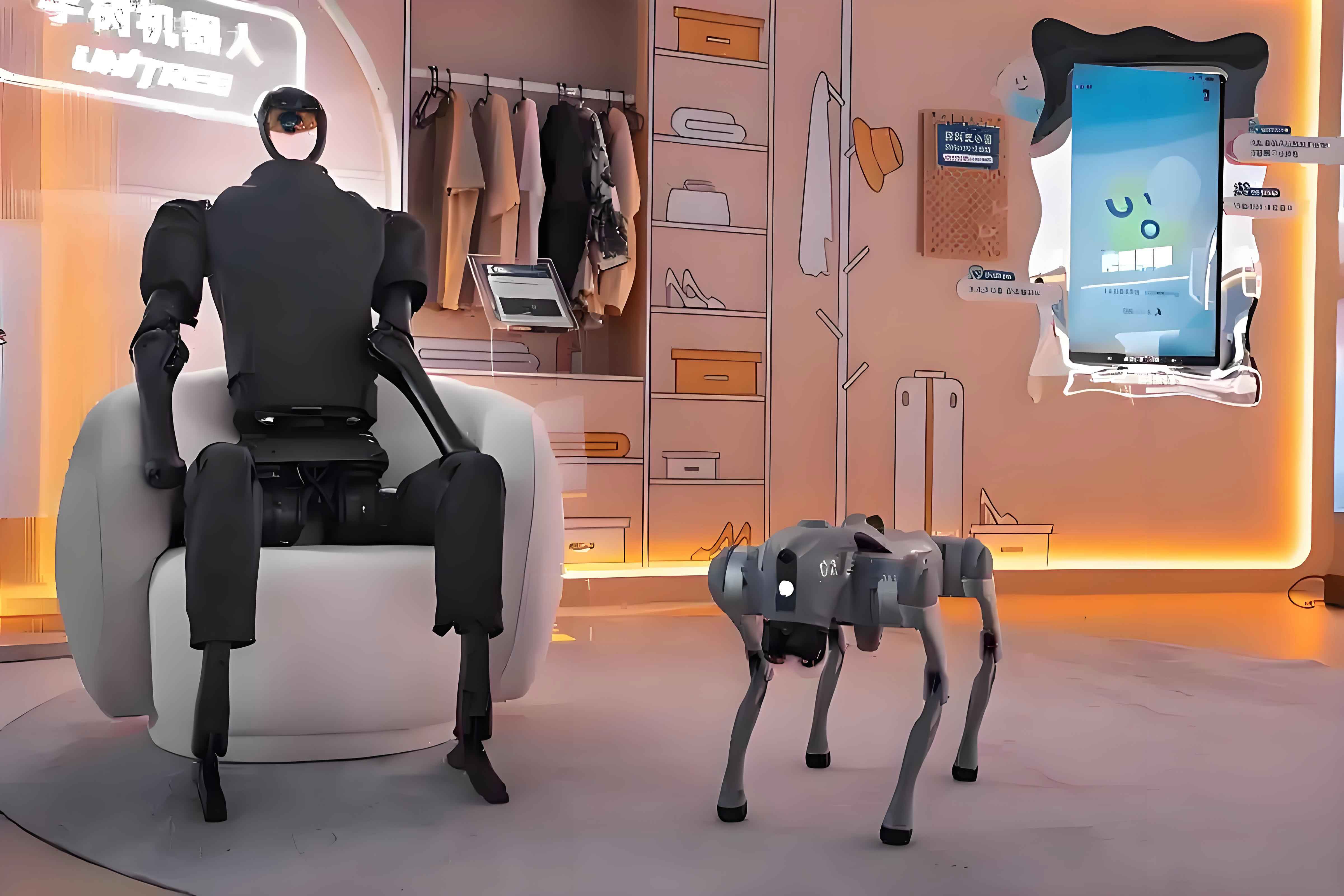
5.1 Hardware and Software Setup
The robot head is equipped with a Jetson Orin NX development platform. The CPU is a 6-core ARM Cortex-A78AE v8.2, and the GPU is a 1024-core NVIDIA Ampere architecture with 32 Tensor Cores. An Intel RealSense D455 depth camera provides synchronized RGB and depth streams at 640×480 resolution and 30 Hz. The camera is connected to the Jetson Orin NX via USB 3.0. The robot has two 15-DOF arms. All algorithms run on an external computer due to the high computational demands of pose estimation, and communication is handled through ROS Noetic.
5.2 System Architecture
The Jetson Orin NX receives RGB-D frames and publishes them over ROS topics. The external computer subscribes to these topics, runs the proposed pipeline, and publishes the estimated object pose. The pose is then sent via EtherCAT to the robot control system, which executes the grasping and pouring tasks.
5.3 Hand-Eye Calibration
The pose estimated by the algorithm is relative to the camera optical center. To transform it to the robot’s head base frame, I performed hand-eye calibration. The transformation from the camera frame to the head base frame is described by the matrix:
$$ \mathbf{A} = \begin{bmatrix} 0.00199 & 0.00142 & 0.99999 & -0.01289 \\ -0.99881 & -0.04868 & 0.00206 & -0.02912 \\ 0.04868 & -0.99881 & 0.00132 & 0.00133 \\ 0 & 0 & 0 & 1 \end{bmatrix} $$
Given a bottle pose in the camera frame, denoted as $\mathbf{B}$, the pose in the head base frame is:
$$ \mathbf{C} = \mathbf{A} \mathbf{B} $$
In one experiment, the measured bottle pose in the camera frame was:
$$ \mathbf{B} = \begin{bmatrix} 9.65107 & 6.89567 & 2.52611 & 8.09751 \\ -2.93452 & 9.87108 & -1.57341 & 1.31985 \\ -2.60205 & 1.44438 & 9.54688 & 3.85774 \\ 0 & 0 & 0 & 1 \end{bmatrix} $$
which resulted in:
$$ \mathbf{C} = \begin{bmatrix} -2.58698 & 1.47210 & 9.54957 & 3.85682 \\ -9.50209 & -7.36501 & -2.42684 & -5.17686 \\ 3.39740 & -9.52174 & 1.70711 & -1.06371 \\ 0 & 0 & 0 & 1 \end{bmatrix} $$
5.4 ROS Communication Protocol
I used ROS topics to synchronize the pipeline with the robot controller. Two boolean topics, bStartGrabBottle and bStartGrabCup, trigger the corresponding recognition tasks. When a trigger is set to true, the pipeline runs the segmentation and pose estimation. The final pose is converted to a translation triple and a rotation quaternion:
$$ t_x = t_1, \quad t_y = t_2, \quad t_z = t_3 $$
and
$$ w = \frac{\sqrt{1 + r_{11} + r_{22} + r_{33}}}{2}, \quad x = \frac{r_{32} – r_{23}}{4w}, \quad y = \frac{r_{13} – r_{31}}{4w}, \quad z = \frac{r_{21} – r_{12}}{4w} $$
These values are published to bottle_pose and cup_pose. After publishing, the system sends saveBottlePose and saveCupPose signals to indicate task completion.
5.5 Experimental Results
The robot was placed in an indoor environment with a water bottle and a cup on a table. The robot first pitched its head to bring the objects into view. After receiving the start signal, the algorithm continuously estimated the pose of the most relevant object according to the mask-area selection strategy. The estimated pose was sent to the controller, which guided the arm to grasp the bottle and then pour water into the cup.
To measure the accuracy, I moved the bottle by 10 cm along each axis and compared the estimated displacement with the true displacement.
| Axis | True displacement (cm) | Predicted displacement (cm) | Error (cm) |
|---|---|---|---|
| x | 10.00 | 9.05 | 0.95 |
| y | 10.00 | 10.88 | 0.88 |
| z | 10.00 | 10.65 | 0.65 |
| Axis | True displacement (cm) | Predicted displacement (cm) | Error (cm) |
|---|---|---|---|
| x | 10.00 | 10.40 | 0.40 |
| y | 10.00 | 10.86 | 0.86 |
| z | 10.00 | 9.88 | 0.12 |
The average error was below 1 cm, which is sufficient for grasping household objects. The hybrid pose estimation mode achieved a frame rate of about 10 Hz, while the pure tracking mode reached 32 Hz. The per-frame estimation mode ran at approximately 2 Hz. The hybrid mode provided the best balance between speed and accuracy for the pouring task.
5.6 Discussion
The experimental results demonstrate that the proposed visual-only pipeline is effective for humanoid robot object manipulation. The use of a YOLOv8-based instance segmentation module provides real-time masks with sufficient quality. The BundleSDF-based reconstruction module allows the robot to create usable 3D models of new objects on the spot. FoundationPose, coupled with the proposed mask and model adaptation, enables accurate 6D pose estimation without per-object training.
One limitation is that transparent objects remain challenging. In my experiments, I used labels and partial reconstruction to reduce the effect of transparency. In future work, I plan to implement more advanced depth completion techniques and to optimize the pipeline for embedded deployment on the Jetson Orin NX itself.
Conclusion
I presented a complete pose estimation pipeline for humanoid robots that relies solely on RGB-D visual input. The pipeline integrates instance segmentation, 3D reconstruction, and 6D pose estimation. I improved the segmentation mask format, the multi-object selection strategy, the centroid calibration, the de-symmetrization of reconstructed models, and the pose estimation scheduling. Extensive real-world experiments on a humanoid robot upper-body platform confirmed that the pipeline can accurately localize and grasp bottles and cups, with pose estimation errors below 1 cm. The results outperform traditional approaches such as DOPE in terms of zero-shot generalization. Future research will focus on model compression, deployment on embedded devices, and robust handling of transparent and reflective objects.