
The accurate real-time knowledge of a robotic manipulator’s end effector pose—comprising both position and orientation—is fundamental for precise task execution in applications ranging from assembly and welding to surgical robotics and autonomous material handling. While kinematic models, such as those derived from Denavit-Hartenberg (D-H) parameters, provide a theoretical framework for calculating this pose, discrepancies between the idealized model and the physical robot are inevitable. These errors stem from multiple sources: geometric parameter inaccuracies (link lengths, joint offsets), non-geometric factors like joint compliance, gear backlash, temperature-induced deformations, and the mechanical load introduced by the end effector tool itself. Crucially, the connection between the robot’s final flange and the end effector often introduces unmodeled offsets and twists. Consequently, the pose calculated through forward kinematics can significantly deviate from the actual pose of the end effector in the workspace, degrading system performance.
To compensate for these errors, external sensing is essential. Vision systems are powerful but can be computationally expensive, sensitive to lighting conditions, and suffer from occlusion. Inertial Measurement Units (IMUs), particularly Micro-Electro-Mechanical Systems (MEMS) based sensors, offer a compelling alternative for direct, real-time attitude (orientation) estimation of the end effector. An IMU, typically containing a tri-axial accelerometer, gyroscope, and magnetometer, provides complementary data: gyroscopes measure angular rate, accelerometers sense specific force (gravity + linear acceleration), and magnetometers sense the Earth’s magnetic field. By fusing these signals, the 3D orientation of the sensor—and thus the end effector to which it is rigidly attached—can be determined.
However, employing an IMU on a dynamic robotic end effector presents distinct challenges. The core assumption for using accelerometers for tilt (roll and pitch) estimation is that the measured specific force is predominantly due to gravity. During slow or static phases of robotic motion, this holds true. However, during dynamic motions involving acceleration or deceleration of the end effector, the accelerometer measures a vector sum of gravitational and kinematic accelerations. Treating this sum as purely gravitational leads to large attitude estimation errors, often referred to as “acceleration disturbances.” Simultaneously, gyroscopes, which are excellent for tracking dynamic rotation, suffer from drift due to bias instability and noise, causing unbounded error growth in orientation if used alone. Therefore, effective sensor fusion is critical to leverage the strengths of each sensor while mitigating their weaknesses.
This article presents a method for optimizing the attitude estimation of a robotic end effector using a MEMS-IMU. The approach strategically divides the manipulator’s operation into static and dynamic phases, applying tailored algorithms for each. For static phases, a direct gravitational acceleration-based method provides a simple and accurate baseline. For dynamic phases, an Adaptive Extended Kalman Filter (AEKF) is designed. The core innovation of this AEKF lies in its ability to dynamically adjust its confidence in the accelerometer and magnetometer measurements based on the magnitude of external acceleration. By statistically characterizing the observed disturbance and adapting the filter’s measurement noise covariance matrix, the algorithm intelligently balances the information from the gyroscope and the aiding sensors, minimizing the corrupting influence of non-gravitational accelerations on the final end effector attitude estimate.
Attitude Representation and Sensor Modeling
To estimate the orientation of the end effector, we first define the necessary coordinate frames. The body frame \( b \) is fixed to the IMU, which is assumed to be securely mounted at the center of the end effector. The reference navigation frame \( n \) is defined as a local East-North-Up (ENU) tangent frame. The attitude of frame \( b \) relative to frame \( n \) can be parameterized using Euler angles (Roll \( \phi \), Pitch \( \theta \), Yaw \( \psi \)), following a specific rotation sequence. For this work, the “Z-X-Y” sequence is used for derivation in dynamic estimation. The relationship between a vector in the navigation frame \( \mathbf{v}^n \) and the body frame \( \mathbf{v}^b \) is given by the direction cosine matrix \( \mathbf{C}_b^n \):
$$ \mathbf{v}^b = \mathbf{C}_b^n \mathbf{v}^n $$
The IMU sensors provide measurements related to this attitude. The tri-axial accelerometer measures specific force \( \mathbf{f}^b \), which is the sum of the kinematic acceleration \( \mathbf{a}^b \) and the gravitational acceleration \( \mathbf{g}^b \) expressed in the body frame, plus measurement noise \( \boldsymbol{\nu}_a \):
$$ \mathbf{f}^b = \mathbf{C}_b^n (\mathbf{a}^n + \mathbf{g}^n) + \boldsymbol{\nu}_a = \mathbf{a}^b + \mathbf{g}^b + \boldsymbol{\nu}_a $$
where \( \mathbf{g}^n = [0, 0, g]^T \) and \( g \) is the local gravity magnitude.
Static Phase Attitude Determination
When the robotic end effector is stationary or moving at a constant velocity (\( \mathbf{a}^n \approx \mathbf{0} \)), the accelerometer measurement simplifies to \( \mathbf{f}^b \approx \mathbf{g}^b + \boldsymbol{\nu}_a \). Ignoring noise, the measured vector points opposite to the local gravity vector. Roll (\( \phi \)) and Pitch (\( \theta \)) can be directly computed from the accelerometer readings \( [f_x, f_y, f_z]^T \):
$$ \theta = \arcsin\left(\frac{f_y}{g}\right), \quad \phi = \arctan2\left(-f_x, f_z\right) $$
With roll and pitch estimated, the tilt-compensated magnetic field vector can be used to calculate Yaw (\( \psi \)). Let \( \mathbf{m}^b = [m_x, m_y, m_z]^T \) be the magnetometer measurement. First, the measured magnetic field is rotated into a level frame using an intermediate DCM \( \mathbf{C}_{b}^{n’} \) constructed from \( \phi \) and \( \theta \):
$$ \mathbf{m}^{n’} = \mathbf{C}_{b}^{n’} \mathbf{m}^b $$
Then, the yaw angle relative to magnetic North is:
$$ \psi = \arctan2(m_{y}^{n’}, m_{x}^{n’}) $$
This method provides an accurate, drift-free attitude estimate for the static end effector, primarily limited by sensor noise and any residual vibrations.
Dynamic Phase Gyroscope Integration and Error Model
During motion, the gyroscope’s angular rate measurements \( \boldsymbol{\tilde{\omega}}^b \) are integrated to propagate attitude. The differential equation for Euler angles (using the Z-X-Y sequence) is:
$$ \dot{\boldsymbol{\Theta}} = \mathbf{\Gamma}(\boldsymbol{\Theta}) \boldsymbol{\omega}_{nb}^b $$
where \( \boldsymbol{\Theta} = [\theta, \phi, \psi]^T \) and \( \boldsymbol{\omega}_{nb}^b \) is the true angular velocity of frame \( b \) relative to frame \( n \), expressed in \( b \). The matrix \( \mathbf{\Gamma}(\boldsymbol{\Theta}) \) is derived from the kinematics of the chosen Euler sequence.
The gyroscope measurement is corrupted by various errors:
$$ \boldsymbol{\tilde{\omega}}^b = \boldsymbol{\omega}_{nb}^b + \mathbf{b}_g + \mathbf{S} \boldsymbol{\omega}_{nb}^b + \mathbf{N} \boldsymbol{\omega}_{nb}^b + \boldsymbol{\varepsilon}_g $$
where:
- \( \mathbf{b}_g \) is the bias vector (slowly varying offset).
- \( \mathbf{S} \) is a diagonal matrix of scale factor errors.
- \( \mathbf{N} \) is a matrix representing non-orthogonality and cross-axis sensitivities.
- \( \boldsymbol{\varepsilon}_g \) is Gaussian white noise.
For a MEMS-IMU on a robotic end effector, bias \( \mathbf{b}_g \) and scale factor \( \mathbf{S} \) are the most significant and variable error sources, highly dependent on temperature and operational conditions. Non-orthogonality \( \mathbf{N} \) is relatively stable and can be calibrated beforehand. Therefore, we construct a state vector for estimation that includes not only the attitude but also these key error parameters to enable online compensation:
$$ \mathbf{x} = \left[ \boldsymbol{\Theta}^T, \mathbf{b}_g^T, \mathbf{s}^T \right]^T $$
where \( \mathbf{s} = [S_x, S_y, S_z]^T \) are the diagonal elements of \( \mathbf{S} \). The continuous-time nonlinear state equation is:
$$ \dot{\mathbf{x}} = \mathbf{f}(\mathbf{x}, \boldsymbol{\tilde{\omega}}^b) + \mathbf{w} $$
where \( \mathbf{w} \) is the process noise, and the function \( \mathbf{f}(\cdot) \) encapsulates the Euler angle kinematics from Eq. (3) using the corrected angular rate \( \boldsymbol{\omega}_{nb}^b = \boldsymbol{\tilde{\omega}}^b – \mathbf{b}_g – \mathbf{S} \boldsymbol{\tilde{\omega}}^b \), with the biases and scale factors assumed to be random constants or slowly varying (modeled as driven by noise).
The measurement model for the Kalman filter uses the roll and pitch calculated from the accelerometer (Eq. 2) and the yaw from the magnetometer (Eq. 4) as observations:
$$ \mathbf{z}_k = \mathbf{H} \mathbf{x}_k + \mathbf{v}_k = \begin{bmatrix} \theta_{acc} \\ \phi_{acc} \\ \psi_{mag} \end{bmatrix}_k + \mathbf{v}_k $$
where \( \mathbf{H} = [\mathbf{I}_{3\times3}, \mathbf{0}_{3\times6}] \) and \( \mathbf{v}_k \) is the measurement noise, with covariance \( \mathbf{R}_k \). The critical challenge is that during dynamic motion of the end effector, \( \theta_{acc} \) and \( \phi_{acc} \) are corrupted by the kinematic acceleration \( \mathbf{a}^b \), making \( \mathbf{v}_k \) non-stationary and significantly larger than during static periods.
Design of the Adaptive Extended Kalman Filter
The standard Extended Kalman Filter (EKF) linearizes the nonlinear system around the current state estimate and performs a two-step prediction and update cycle. The prediction step uses the gyroscope data to propagate the state and its error covariance \( \mathbf{P} \):
$$ \hat{\mathbf{x}}_k^- = \hat{\mathbf{x}}_{k-1}^+ + \mathbf{f}(\hat{\mathbf{x}}_{k-1}^+, \boldsymbol{\tilde{\omega}}^b_{k-1}) \Delta t $$
$$ \mathbf{P}_k^- = \mathbf{\Phi}_k \mathbf{P}_{k-1}^+ \mathbf{\Phi}_k^T + \mathbf{Q}_k $$
where \( \mathbf{\Phi}_k \approx \mathbf{I} + \mathbf{F}(\hat{\mathbf{x}}_{k-1}^+) \Delta t \) is the discrete state transition matrix from linearizing \( \mathbf{f} \), and \( \mathbf{Q}_k \) is the process noise covariance matrix.
The update step corrects the prediction using the sensor observations:
$$ \mathbf{K}_k = \mathbf{P}_k^- \mathbf{H}^T (\mathbf{H} \mathbf{P}_k^- \mathbf{H}^T + \mathbf{R}_k)^{-1} $$
$$ \hat{\mathbf{x}}_k^+ = \hat{\mathbf{x}}_k^- + \mathbf{K}_k (\mathbf{z}_k – \mathbf{H} \hat{\mathbf{x}}_k^-) $$
$$ \mathbf{P}_k^+ = (\mathbf{I} – \mathbf{K}_k \mathbf{H}) \mathbf{P}_k^- $$
The Kalman gain \( \mathbf{K}_k \) determines the weight given to the new measurement \( \mathbf{z}_k \). It is inversely proportional to the measurement noise covariance \( \mathbf{R}_k \). In a conventional EKF, \( \mathbf{R}_k \) is fixed based on the static noise characteristics of the accelerometer and magnetometer. This is problematic for a robotic end effector because during dynamic acceleration, the actual error in \( \theta_{acc} \) and \( \phi_{acc} \) far exceeds the static noise level. Using a fixed \( \mathbf{R} \) causes the filter to over-trust the erroneous accelerometer data, leading to large attitude errors.
Adaptive Measurement Noise Covariance Estimation
The proposed adaptive algorithm dynamically adjusts \( \mathbf{R}_k \) based on the magnitude of external acceleration experienced by the end effector. The core idea is to detect when the accelerometer data is unreliable for tilt estimation and to proportionally increase the corresponding elements in \( \mathbf{R}_k \), thereby reducing the Kalman gain \( \mathbf{K}_k \) and the influence of the corrupt measurement on the state update.
The external acceleration magnitude \( a_{ext} \) is estimated as the deviation of the accelerometer reading from gravity:
$$ a_{ext} = ||\, \mathbf{f}^b – \mathbf{g}^b(\hat{\boldsymbol{\Theta}}^-) \,|| $$
where \( \mathbf{g}^b(\hat{\boldsymbol{\Theta}}^-) \) is the gravity vector predicted in the body frame using the attitude estimate from the filter’s prediction step \( \hat{\boldsymbol{\Theta}}^- \).
The adaptive algorithm then modifies the measurement noise covariance matrix \( \mathbf{R}_k \) as follows:
- Static/Low-Acceleration Regime: If \( a_{ext} \leq \sigma_a \), where \( \sigma_a \) is the empirical standard deviation of accelerometer noise during static conditions, the end effector is considered quasi-static. The measurement is trusted, and \( \mathbf{R}_k \) is set to its baseline value \( \mathbf{R}_0 \), which is diagonal with elements \( (\sigma_{\theta}^2, \sigma_{\phi}^2, \sigma_{\psi}^2) \) determined from static sensor calibration.
$$ \mathbf{R}_k = \mathbf{R}_0 = \begin{bmatrix} \sigma_{\theta}^2 & 0 & 0 \\ 0 & \sigma_{\phi}^2 & 0 \\ 0 & 0 & \sigma_{\psi}^2 \end{bmatrix} $$ - Moderate-Acceleration Regime: If \( \sigma_a < a_{ext} \leq a_{th} \), where \( a_{th} \) is a pre-defined high-acceleration threshold (e.g., \( 0.5g \)), the external acceleration is deemed significant enough to corrupt tilt sensing. The variance for the roll and pitch observations is increased proportionally to \( a_{ext}^2 \). The yaw observation variance is also increased, but based on the tilt error induced by acceleration \( (a_{ext}/g) \).
$$ \mathbf{R}_k = \mathbf{R}_0 + \begin{bmatrix} k_1 \cdot a_{ext}^2 & 0 & 0 \\ 0 & k_1 \cdot a_{ext}^2 & 0 \\ 0 & 0 & k_2 \cdot (a_{ext}/g)^2 \end{bmatrix} $$
Here, \( k_1 \) and \( k_2 \) are tuning parameters that scale the added variance. - High-Acceleration Regime: If \( a_{ext} > a_{th} \), the kinematic acceleration is very high, and the accelerometer/magnetometer data is considered too unreliable to aid the filter. Effectively, the filter should rely solely on the gyroscope propagation. This is achieved by setting the observation variances to an extremely large value \( \sigma_{se}^2 \), which drives the Kalman gain \( \mathbf{K}_k \) near zero.
$$ \mathbf{R}_k = \begin{bmatrix} \sigma_{se}^2 & 0 & 0 \\ 0 & \sigma_{se}^2 & 0 \\ 0 & 0 & \sigma_{se}^2 \end{bmatrix} $$
This adaptive mechanism allows the filter to seamlessly transition between trusting the aiding sensors during slow, precise movements of the end effector and relying on the short-term accuracy of the gyroscopes during fast, dynamic motions, all while continuously estimating and compensating for gyro bias and scale factor errors.
Experimental Validation and Results
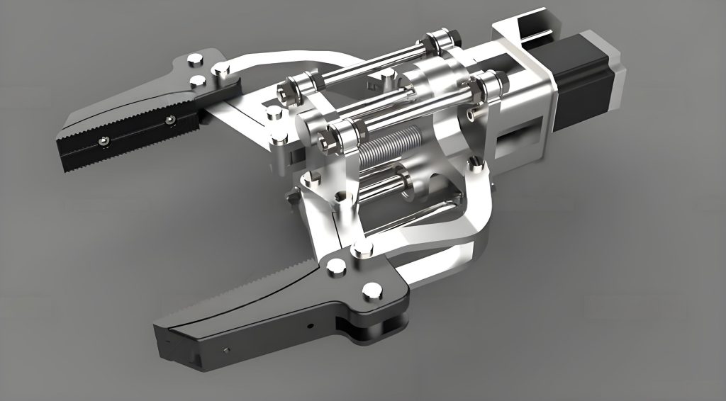
The proposed system was validated using a 6-degree-of-freedom industrial robotic arm. A MEMS-based 9-axis IMU (MPU-9250) was securely attached to the center of a two-finger gripper acting as the end effector. The IMU data was sampled at 100 Hz. The robot’s controller provided joint angles, which were used with the nominal D-H parameters to compute the forward kinematics as a baseline reference for the end effector’s orientation. It is important to note that this kinematic estimate contains the very errors the IMU aims to compensate for, but it serves as a consistent trajectory reference. The primary evaluation focuses on the IMU’s ability to provide a stable, accurate, and drift-corrected attitude estimate.
Static Alignment and Calibration
Initially, the end effector was placed in a known orientation (defined as \( [0^\circ, 0^\circ, 0^\circ] \) for Roll, Pitch, Yaw). IMU data was collected for two minutes while static. The average of the accelerometer and magnetometer readings over this period was used with the static algorithm (Eq. 2 & 4) to determine the initial attitude offset between the IMU frame and the robot’s nominal end effector frame. This offset, primarily due to the mounting of the gripper, was calculated and used to align all subsequent IMU estimates to the robot’s coordinate system. The residual error after this alignment was minimal, confirming the accuracy of the static calibration method for the end effector’s initial state.
Static Point-to-Point Motion
The robot was commanded to move sequentially through five distinct poses, dwelling at each for 2 seconds. During the dwell periods, the static attitude algorithm was applied. The estimated orientations were compared against the orientations derived from the robot’s forward kinematics at those taught points. The results, shown in the table below, demonstrate excellent agreement. The small residual errors are attributed to a combination of static sensor noise, minor vibrations, and the fundamental geometric parameter errors in the robot’s kinematic model that the IMU naturally bypasses.
| Target Point | Roll Error (°) | Pitch Error (°) | Yaw Error (°) |
|---|---|---|---|
| 1 | 0.05 | -0.04 | 0.23 |
| 2 | 0.09 | 0.03 | 0.15 |
| 3 | -0.02 | 0.04 | 0.29 |
| 4 | 0.12 | -0.06 | 0.12 |
| 5 | 0.06 | 0.05 | 0.19 |
| Average | 0.06 | 0.00 | 0.20 |
Dynamic Motion: Constant Velocity
The end effector was commanded to follow a smooth, constant-velocity trajectory. Since the motion involved minimal acceleration, the external acceleration \( a_{ext} \) remained small. Both the standard EKF (with fixed \( \mathbf{R} \)) and the proposed AEKF were executed. As expected, both filters performed well, with attitude errors staying within a small bound. The AEKF showed marginally better performance, primarily due to its online estimation and compensation of gyroscope bias, which slightly improves long-term drift characteristics even in low-acceleration scenarios.
| Algorithm | Roll Error (°) | Pitch Error (°) | Yaw Error (°) |
|---|---|---|---|
| Standard EKF | 0.27 | 0.54 | -0.78 |
| Proposed AEKF | 0.34 | 0.36 | -0.35 |
Dynamic Motion: Variable Acceleration
This experiment was designed to stress the system. The end effector was commanded through a trajectory involving periods of high acceleration and deceleration. The performance difference between the standard EKF and the AEKF became starkly evident. The standard EKF, trusting the accelerometer equally at all times, exhibited large transient errors whenever the end effector accelerated. These errors appeared as spikes in the estimated roll and pitch angles. In contrast, the AEKF successfully detected these high-acceleration phases via the \( a_{ext} \) metric. It automatically inflated the measurement noise covariance \( \mathbf{R}_k \), thereby reducing the corrupting influence of the accelerometer data and relying more on the propagated state from the (bias-compensated) gyroscopes. The result was a dramatically smoother and more accurate attitude estimate throughout the aggressive motion.
The quantitative improvement is summarized in the table below, showing the root-mean-square error (RMSE) for a representative high-acceleration segment of the trajectory. The AEKF reduces the attitude error by a significant margin, particularly for roll and pitch which are directly affected by linear acceleration.
| Algorithm | Roll RMSE (°) | Pitch RMSE (°) | Yaw RMSE (°) |
|---|---|---|---|
| Standard EKF | 4.72 | 2.15 | 1.98 |
| Proposed AEKF | 1.85 | 1.02 | 1.45 |
| Improvement | 2.87° | 1.13° | 0.53° |
Conclusion
Accurate real-time attitude estimation for a robotic end effector is critical for closing the gap between commanded and actual pose. This work has presented a robust, IMU-based solution that effectively compensates for errors arising from joint compliance, kinematic model inaccuracies, and the end effector attachment itself. The method employs a dual-strategy approach: a simple, accurate static algorithm for slow movements, and an innovative Adaptive Extended Kalman Filter for dynamic operation.
The key contribution is the adaptive mechanism that modifies the filter’s measurement update based on the magnitude of external acceleration detected at the end effector. By dynamically adjusting the confidence in the accelerometer and magnetometer data, the algorithm effectively mitigates the largest source of error in IMU-based attitude estimation during robotic manipulation tasks. Experimental results on a 6-DOF robotic arm demonstrate that the proposed AEKF significantly outperforms a standard EKF during motions involving acceleration, leading to a more stable and precise estimate of the end effector’s orientation. This enhanced situational awareness of the end effector’s attitude can directly improve the accuracy of force control, path following, and compliant manipulation, enabling higher performance in advanced robotic applications.
Future work may involve tightly coupling this IMU-based attitude estimate with the robot’s joint encoder data in a sensor fusion framework to also improve the Cartesian position estimate of the end effector, and to potentially enable online calibration of the robot’s kinematic parameters.