
In the field of robotics and precision machinery, the demand for high-performance and reliable components has grown significantly. Among these, the RV reducer (Rotary Vector reducer) plays a pivotal role as a key transmission component in industrial robots, directly influencing motion accuracy, load capacity, and operational stability. The assembly process of an RV reducer is complex, involving numerous parts such as the pin gear housing, cycloid gears, crankshafts, and pin pins. Traditional manual selective assembly methods often lead to inconsistencies in matching quality, resulting in suboptimal transmission accuracy, low assembly success rates, and increased production costs due to trial and error. To address these challenges, we propose a novel selective assembly scheme for RV reducers based on an improved genetic algorithm. This scheme aims to maximize the number of successfully assembled RV reducers in batch production while ensuring optimal transmission precision, thereby improving overall efficiency and product quality.
The core of our approach lies in formulating the selective assembly problem as a combinatorial optimization task in discrete space, where the goal is to select and group parts from different categories to meet stringent precision constraints. We develop a mathematical model that incorporates the structural characteristics and transmission principles of the RV reducer, accounting for various error terms from critical components. To solve this model efficiently, we enhance the traditional genetic algorithm by integrating simulated annealing principles and adaptive adjustment strategies, leading to faster convergence and enhanced global search capabilities. Our improved algorithm, referred to as SAGA (Simulated Annealing and Adaptive Genetic Algorithm), employs integer encoding for chromosomes, modified crossover and mutation operations tailored to the RV reducer’s assembly requirements, and a tournament selection mechanism infused with simulated annealing to maintain population diversity. Through extensive experiments, we demonstrate that SAGA outperforms conventional genetic algorithms and other variants in terms of matching success rates and solution quality, offering a robust and practical solution for high-precision RV reducer manufacturing.
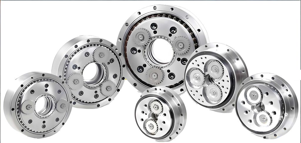
The RV reducer, particularly the RV-20E type, consists of multiple precision components that must be assembled with minimal clearance and alignment errors to achieve high transmission accuracy. The transmission error, a critical performance metric, is influenced by manufacturing tolerances and assembly deviations. Key parts include the pin gear housing, cycloid gears, crankshafts, and pin pins, each contributing specific error terms. For instance, the pin gear housing introduces errors in center circle diameter, base circle diameter, and pin hole position; cycloid gears have errors in bore diameter, base circle diameter, cumulative pitch, and radial runout; crankshafts have errors in shaft diameters; and pin pins have diameter variations. These errors interact during assembly, affecting the overall transmission error. Therefore, selective assembly involves choosing specific parts from each category to form sets that collectively minimize the transmission error within acceptable limits.
To model this problem mathematically, we consider a batch of n sets of parts available for selective assembly. Each part is categorized and assigned a unique identifier. Let the error set for pin gear housings be denoted as H, for cycloid gears as C, for crankshafts as B, and for pin pins as P. Specifically, for the i-th pin gear housing, the errors are represented as a tuple: $$H_i = (h_{1,i}, h_{2,i}, h_{3,i})$$ where \(h_{1,i}\) is the center circle diameter error, \(h_{2,i}\) is the base circle diameter error, and \(h_{3,i}\) is the pin hole position error. Similarly, for cycloid gears, the error tuple is: $$C_j = (c_{1,j}, c_{2,j}, c_{3,j}, c_{4,j}, c_{5,j})$$ where \(c_{1,j}\) and \(c_{2,j}\) are bore diameter errors, \(c_{3,j}\) is the base circle diameter error, \(c_{4,j}\) is the cumulative pitch error, and \(c_{5,j}\) is the radial runout error. For crankshafts: $$B_k = (b_{1,k}, b_{2,k})$$ with \(b_{1,k}\) and \(b_{2,k}\) as shaft diameter errors. Pin pins are classified into two types with fixed diameter errors \(p_1\) and \(p_2\). The ranges for these errors, based on the RV-20E reducer specifications, are summarized in Table 1.
| Error Symbol | Range (μm) |
|---|---|
| \(h_{1,i}\) | [-5, 5] |
| \(h_{2,i}\) | [-6, 6] |
| \(h_{3,i}\) | [0, 4] |
| \(c_{1,i}, c_{2,i}\) | [-17, -7] |
| \(c_{3,i}\) | [-3, 7] |
| \(c_{4,i}\) | [0, 8] |
| \(c_{5,i}\) | [0, 7] |
| \(b_{1,i}, b_{2,i}\) | [-17, -7] |
| \(p_1\) | -1 |
| \(p_2\) | -2 |
In selective assembly, we aim to form a pre-assembly scheme S consisting of n potential RV reducer sets, where each set \(s_x\) includes one pin gear housing, two cycloid gears, two crankshafts, and one pin pin. The transmission error for each set is computed based on the interplay of part errors. Let \(s_x\) be composed of pin gear housing g, cycloid gears i and j, crankshafts m and n, and pin pin type l. The transmission error \(\delta_x\) is split into two components, \(\delta_{1,x}\) and \(\delta_{2,x}\), corresponding to the two stages of the RV reducer’s transmission. The constraints are defined as follows:
$$ \delta_{1,x} = 0.001 \cdot \left\{ \alpha_1 \cdot h_{1,g} + \alpha_2 \cdot \min[(c_{1,i} – b_{1,m}), (c_{2,i} – b_{1,n})] + \alpha_3 \cdot (h_{2,g} – c_{3,i} – p_l) + \alpha_4 \cdot (2h_{3,g} – c_{4,i}) + \alpha_5 \cdot c_{5,i} \right\} $$
$$ \delta_{2,x} = 0.001 \cdot \left\{ \alpha_1 \cdot h_{1,g} + \alpha_2 \cdot \min[(c_{2,j} – b_{2,m}), (c_{1,j} – b_{2,n})] + \alpha_3 \cdot (h_{2,g} – c_{3,j} – p_l) + \alpha_4 \cdot (2h_{3,g} – c_{4,j}) + \alpha_5 \cdot c_{5,j} \right\} $$
Subject to:
$$ \Delta_{\text{min}} \leq \delta_{1,x} \leq \Delta_{\text{max}}, \quad \Delta_{\text{min}} \leq \delta_{2,x} \leq \Delta_{\text{max}} $$
$$ \text{CB}_{\text{min}} \leq c_{1,i} – b_{1,m} \leq \text{CB}_{\text{max}}, \quad \text{CB}_{\text{min}} \leq c_{2,i} – b_{1,n} \leq \text{CB}_{\text{max}} $$
$$ \text{CB}_{\text{min}} \leq c_{2,j} – b_{2,m} \leq \text{CB}_{\text{max}}, \quad \text{CB}_{\text{min}} \leq c_{1,j} – b_{2,n} \leq \text{CB}_{\text{max}} $$
$$ \text{HCP}_{\text{min}} \leq h_{2,g} – c_{3,i} – p_l \leq \text{HCP}_{\text{max}}, \quad \text{HCP}_{\text{min}} \leq h_{2,g} – c_{3,j} – p_l \leq \text{HCP}_{\text{max}} $$
$$ \text{HC}_{\text{min}} \leq 2h_{3,g} – c_{4,i} \leq \text{HC}_{\text{max}}, \quad \text{HC}_{\text{min}} \leq 2h_{3,g} – c_{4,j} \leq \text{HC}_{\text{max}} $$
Here, \(\Delta_{\text{max}}\) and \(\Delta_{\text{min}}\) are the upper and lower limits for transmission error, while \(\text{CB}_{\text{max}}\), \(\text{CB}_{\text{min}}\), \(\text{HCP}_{\text{max}}\), \(\text{HCP}_{\text{min}}\), \(\text{HC}_{\text{max}}\), and \(\text{HC}_{\text{min}}\) are bounds for error difference terms between parts. The coefficients \(\alpha_1\) to \(\alpha_5\) are transmission coefficients derived from the RV reducer’s geometry: $$\alpha_1 = \frac{1 – k_c^2}{e_b n_c} \cdot \frac{180 \times 60}{\pi}, \quad \alpha_2 = \frac{180 \times 60}{\pi d_c}, \quad \alpha_3 = \frac{180 \times 60}{\pi e_b n_c}, \quad \alpha_4 = k_c \cdot \frac{180 \times 60}{\pi e_b n_c}, \quad \alpha_5 = \frac{180 \times 60}{2\pi e_b n_c}$$ where \(e_b\) is the crankshaft eccentricity, \(n_c\) is the number of cycloid gear teeth, \(d_c\) is the pitch circle diameter of cycloid gear bores, and \(k_c = e_b n_c / r_h\) with \(r_h\) as the pin gear housing center circle radius. For the RV-20E reducer, typical values are \(e_b = 0.9 \text{ mm}\), \(d_c = 27.5 \text{ mm}\), \(r_h = 52 \text{ mm}\), and \(n_c = 39\). The limits for error differences and transmission error are given in Table 2.
| Parameter | CB (μm) | HCP (μm) | HC (μm) | Δ (°) |
|---|---|---|---|---|
| Upper Limit (max) | 5 | 5 | 5 | 1/60 |
| Lower Limit (min) | 0 | 1 | 0 | 0 |
The objective function for a pre-assembly scheme S is to maximize the number of successfully assembled RV reducer sets. We define an evaluation function for each set \(s_x\): $$ f(s_x) = \begin{cases} 1 & \text{if } \Delta_{\text{min}} \leq \delta_{1,x}, \delta_{2,x} \leq \Delta_{\text{max}} \\ 0 & \text{otherwise} \end{cases} $$ Then, the overall fitness of scheme S is: $$ F(S) = \max \sum_{x=1}^{n} f(s_x) $$ This represents the total number of RV reducer sets that meet the transmission accuracy requirements. The selective assembly problem is thus a high-dimensional combinatorial optimization challenge, as the solution space grows exponentially with n. For n sets of parts, the total number of combinations is approximately \(2n^3(n-1)^2\), which for n=20 is about \(5.78 \times 10^6\), and for n=50 exceeds \(6.0 \times 10^8\). Traditional exhaustive search methods are infeasible, necessitating intelligent optimization algorithms.
To solve this problem efficiently, we propose an improved genetic algorithm, SAGA, which enhances the standard genetic algorithm (GA) by incorporating simulated annealing and adaptive strategies. Genetic algorithms are well-suited for combinatorial optimization due to their population-based search and ability to explore large solution spaces. However, standard GAs often suffer from premature convergence and slow convergence rates. Our improvements address these issues specifically for the RV reducer selective assembly context.
First, we employ integer encoding for chromosomes. Each chromosome represents a potential assembly scheme S, with genes arranged in segments corresponding to individual RV reducer sets. For n sets, a chromosome consists of n segments, each containing 6 gene points: the first point stores the pin gear housing part number, the second point stores the pin pin type, the third and fourth points store cycloid gear part numbers, and the fifth and sixth points store crankshaft part numbers. Part numbers are unique within each category, starting from 1. This encoding ensures that each part is used exactly once per scheme, adhering to the assembly constraints.
The fitness function is directly derived from the objective function: $$ \text{Fit}(S) = \sum_{x=1}^{n} f(s_x) $$ Higher fitness values indicate better schemes with more successfully assemblable RV reducers. The genetic operations—selection, crossover, and mutation—are tailored to maintain feasibility and improve search efficiency.
For selection, we use a tournament selection mechanism enhanced with simulated annealing principles. Instead of always selecting the individual with higher fitness, we introduce a probability based on the Metropolis criterion from simulated annealing. In each tournament, two individuals are randomly chosen from the population. Let their fitness values be \(\text{Fit}_1\) and \(\text{Fit}_2\). The probability of selecting the first individual is: $$ p_s = \begin{cases} 1 & \text{if } \text{Fit}_1 \geq \text{Fit}_2 \\ \exp\left(\frac{\text{Fit}_1 – \text{Fit}_2}{T}\right) & \text{if } \text{Fit}_1 < \text{Fit}_2 \end{cases} $$ where T is the current temperature, initialized as \(T_0 = 3000\) and decreased by a cooling factor \(q = 0.9\) each generation: \(T = T_0 \cdot q^{\text{generation}}\). This approach helps maintain population diversity and prevents early convergence to local optima. Additionally, we employ an elitist strategy to preserve the best individual across generations.
Crossover is a critical operation for generating new offspring. Standard crossover methods like single-point crossover can lead to infeasible solutions where part numbers are duplicated or missing. Therefore, we design a modified crossover operation. Two parent individuals \(S_1\) and \(S_2\) are selected, and a random gene segment (corresponding to one RV reducer set) is chosen as the crossover region. For each gene point in this region, we identify the part number from the other parent at the same position. Then, in the current parent, we locate the gene point with that part number (within the same part category) and swap the values. This ensures that after crossover, each part number appears exactly once in each individual, preserving the assembly constraints. The process is illustrated in Figure 3 (though no figure reference is included in text, we describe it conceptually). This tailored crossover facilitates effective exploration of the solution space while maintaining feasibility.
Mutation introduces random changes to promote diversity. We implement a part-type-based mutation operation. For an individual selected for mutation with probability \(p_m\), we randomly choose two gene segments (representing two RV reducer sets) and a random gene point index (1 to 6). Then, we swap the part numbers at that gene point between the two segments. This essentially exchanges parts of the same type between different RV reducer sets, potentially improving the overall matching without violating part uniqueness. Mutation probability is adaptively adjusted as described below.
To balance exploration and exploitation, we incorporate adaptive adjustment strategies for crossover probability \(p_c\) and mutation probability \(p_m\). Instead of fixed values, these probabilities change based on population diversity, measured by the standard deviation of fitness values. Let \(\sigma_i\) be the standard deviation of fitness in generation i, and \(\sigma_0\) be the standard deviation in the initial population. The adaptive formulas are:
$$ p_c = \begin{cases} p_{cl} & \text{if } p_{cl} \geq p_{cm} \cdot \frac{\sigma_i}{\sigma_0} \\ p_{cm} \cdot \frac{\sigma_i}{\sigma_0} & \text{if } p_{cl} < p_{cm} \cdot \frac{\sigma_i}{\sigma_0} < p_{cr} \\ p_{cr} & \text{if } p_{cr} \leq p_{cm} \cdot \frac{\sigma_i}{\sigma_0} \end{cases} $$
$$ p_m = \begin{cases} p_{ml} & \text{if } p_{ml} \geq p_{mm} \cdot \frac{\sigma_0}{\sigma_i} \\ p_{mm} \cdot \frac{\sigma_0}{\sigma_i} & \text{if } p_{ml} < p_{mm} \cdot \frac{\sigma_0}{\sigma_i} < p_{mr} \\ p_{mr} & \text{if } p_{mr} \leq p_{mm} \cdot \frac{\sigma_0}{\sigma_i} \end{cases} $$
where \(p_{cm} = 0.9\), \(p_{cr} = 0.5\), \(p_{cl} = 0.75\) are the initial, upper, and lower bounds for crossover probability, and \(p_{mm} = 0.05\), \(p_{mr} = 0.1\), \(p_{ml} = 0.01\) are those for mutation probability. The standard deviation is computed as: $$ \sigma_i = \sqrt{\frac{1}{N} \sum_{j=1}^{N} (\text{Fit}(j) – \text{Fit}_{\text{avg}})^2 } $$ with N being the population size (set to 20), and \(\text{Fit}_{\text{avg}}\) the average fitness. Early in evolution, when \(\sigma_i\) is high (diverse population), \(p_c\) tends to be lower and \(p_m\) higher to encourage exploration. Later, as diversity decreases, \(p_c\) increases and \(p_m\) decreases to exploit good solutions. This dynamic adjustment enhances convergence speed and global search capability.
The overall SAGA algorithm flowchart is as follows: initialize population with random feasible chromosomes; evaluate fitness; while termination condition (e.g., maximum generations \(M = 10^7\)) not met, do: perform tournament selection with simulated annealing; apply adaptive crossover and mutation to generate offspring; evaluate offspring fitness; combine parents and offspring, select best individuals for next generation (elitism); update temperature T; repeat. This process efficiently searches for optimal RV reducer assembly schemes.
To validate our SAGA algorithm, we conduct experiments with different batch sizes: 10, 20, and 50 sets of RV reducer parts. The part error data are generated based on the ranges in Table 1, ensuring that in an ideal shuffled state, a 100% matching success rate is theoretically achievable (i.e., all n sets can be assembled successfully). We compare SAGA against two baseline algorithms: standard genetic algorithm (GA) and a genetic algorithm with simulated annealing only (SGA). All algorithms use the same population size (20), maximum generations (10^7), and similar operator designs, except for the enhancements in SAGA. Each experiment is run 50 times independently to ensure statistical reliability. The key performance metrics are the number of successfully matched RV reducer sets (success count), matching success rate (success count / n × 100%), and average runtime. The algorithm parameters are summarized in Table 3.
| Parameter | Symbol | Value |
|---|---|---|
| Population Size | N | 20 |
| Maximum Generations | M | 1.0 × 10⁷ |
| Crossover Probability Initial | \(p_{cm}\) | 0.9 |
| Crossover Probability Upper | \(p_{cr}\) | 0.5 |
| Crossover Probability Lower | \(p_{cl}\) | 0.75 |
| Mutation Probability Initial | \(p_{mm}\) | 0.05 |
| Mutation Probability Upper | \(p_{mr}\) | 0.1 |
| Mutation Probability Lower | \(p_{ml}\) | 0.01 |
| Simulated Annealing Initial Temperature | \(T_0\) | 3000 |
| Simulated Annealing Cooling Factor | q | 0.9 |
For the 20-set case, we present detailed part error data in Table 4. This data represents shuffled parts where each part’s errors are within specified ranges, and the optimal assembly should yield 20 successful RV reducers.
| Part Type | Index | Error Values (μm or as noted) |
|---|---|---|
| Pin Gear Housing | 1 | \(h_1=-3, h_2=-1, h_3=4\) |
| 2 | \(h_1=-3, h_2=-2, h_3=4\) | |
| 3 | \(h_1=-1, h_2=2, h_3=4\) | |
| 4 | \(h_1=5, h_2=4, h_3=3\) | |
| 5 | \(h_1=-5, h_2=2, h_3=2\) | |
| 6 | \(h_1=1, h_2=1, h_3=2\) | |
| 7 | \(h_1=-3, h_2=1, h_3=2\) | |
| 8 | \(h_1=-3, h_2=-1, h_3=3\) | |
| 9 | \(h_1=-5, h_2=2, h_3=2\) | |
| 10 | \(h_1=0, h_2=2, h_3=4\) | |
| 11 | \(h_1=-1, h_2=1, h_3=2\) | |
| 12 | \(h_1=-2, h_2=3, h_3=2\) | |
| 13 | \(h_1=-1, h_2=3, h_3=4\) | |
| 14 | \(h_1=-5, h_2=1, h_3=0\) | |
| 15 | \(h_1=-4, h_2=6, h_3=2\) | |
| 16 | \(h_1=-1, h_2=-1, h_3=2\) | |
| 17 | \(h_1=-3, h_2=-3, h_3=3\) | |
| 18 | \(h_1=-1, h_2=1, h_3=3\) | |
| 19 | \(h_1=-2, h_2=4, h_3=3\) | |
| 20 | \(h_1=-1, h_2=5, h_3=3\) | |
| Cycloid Gears | 1 | \(c_1=-12, c_2=-10, c_3=5, c_4=4, c_5=7\) |
| 2 | \(c_1=-10, c_2=-13, c_3=5, c_4=4, c_5=5\) | |
| 3 | \(c_1=-15, c_2=-14, c_3=-2, c_4=6, c_5=2\) | |
| 4 | \(c_1=-8, c_2=-15, c_3=1, c_4=3, c_5=5\) | |
| 5 | \(c_1=-14, c_2=-7, c_3=3, c_4=8, c_5=0\) | |
| 6 | \(c_1=-13, c_2=-12, c_3=-1, c_4=4, c_5=5\) | |
| 7 | \(c_1=-11, c_2=-9, c_3=0, c_4=7, c_5=3\) | |
| 8 | \(c_1=-7, c_2=-7, c_3=1, c_4=3, c_5=4\) | |
| 9 | \(c_1=-9, c_2=-8, c_3=0, c_4=0, c_5=7\) | |
| 10 | \(c_1=-12, c_2=-12, c_3=2, c_4=4, c_5=3\) | |
| 11 | \(c_1=-8, c_2=-11, c_3=-1, c_4=0, c_5=2\) | |
| 12 | \(c_1=-14, c_2=-11, c_3=-2, c_4=2, c_5=2\) | |
| 13 | \(c_1=-8, c_2=-7, c_3=0, c_4=3, c_5=3\) | |
| 14 | \(c_1=-10, c_2=-13, c_3=-1, c_4=0, c_5=2\) | |
| 15 | \(c_1=-11, c_2=-8, c_3=7, c_4=2, c_5=1\) | |
| 16 | \(c_1=-7, c_2=-10, c_3=5, c_4=2, c_5=4\) | |
| 17 | \(c_1=-13, c_2=-8, c_3=3, c_4=3, c_5=5\) | |
| 18 | \(c_1=-8, c_2=-12, c_3=1, c_4=5, c_5=7\) | |
| 19 | \(c_1=-8, c_2=-14, c_3=0, c_4=7, c_5=4\) | |
| 20 | \(c_1=-11, c_2=-12, c_3=2, c_4=1, c_5=7\) | |
| 21 | \(c_1=-14, c_2=-15, c_3=-2, c_4=2, c_5=4\) | |
| 22 | \(c_1=-9, c_2=-16, c_3=-1, c_4=5, c_5=6\) | |
| 23 | \(c_1=-15, c_2=-8, c_3=0, c_4=5, c_5=6\) | |
| 24 | \(c_1=-8, c_2=-11, c_3=4, c_4=5, c_5=0\) | |
| 25 | \(c_1=-7, c_2=-11, c_3=2, c_4=3, c_5=6\) | |
| 26 | \(c_1=-8, c_2=-12, c_3=0, c_4=8, c_5=5\) | |
| 27 | \(c_1=-15, c_2=-11, c_3=2, c_4=5, c_5=5\) | |
| 28 | \(c_1=-12, c_2=-7, c_3=-1, c_4=4, c_5=0\) | |
| 29 | \(c_1=-13, c_2=-12, c_3=1, c_4=7, c_5=6\) | |
| 30 | \(c_1=-13, c_2=-8, c_3=1, c_4=3, c_5=4\) | |
| 31 | \(c_1=-12, c_2=-13, c_3=4, c_4=5, c_5=6\) | |
| 32 | \(c_1=-7, c_2=-13, c_3=2, c_4=3, c_5=7\) | |
| 33 | \(c_1=-11, c_2=-8, c_3=-3, c_4=4, c_5=4\) | |
| 34 | \(c_1=-11, c_2=-13, c_3=-2, c_4=5, c_5=6\) | |
| 35 | \(c_1=-13, c_2=-10, c_3=-2, c_4=3, c_5=6\) | |
| 36 | \(c_1=-10, c_2=-16, c_3=-3, c_4=4, c_5=3\) | |
| 37 | \(c_1=-12, c_2=-15, c_3=-1, c_4=6, c_5=2\) | |
| 38 | \(c_1=-10, c_2=-13, c_3=2, c_4=3, c_5=3\) | |
| 39 | \(c_1=-12, c_2=-15, c_3=5, c_4=4, c_5=3\) | |
| 40 | \(c_1=-12, c_2=-11, c_3=3, c_4=0, c_5=4\) | |
| Crankshafts | 1 | \(b_1=-12, b_2=-13\) |
| 2 | \(b_1=-16, b_2=-9\) | |
| 3 | \(b_1=-10, b_2=-13\) | |
| 4 | \(b_1=-13, b_2=-7\) | |
| 5 | \(b_1=-14, b_2=-13\) | |
| 6 | \(b_1=-13, b_2=-8\) | |
| 7 | \(b_1=-10, b_2=-8\) | |
| 8 | \(b_1=-12, b_2=-16\) | |
| 9 | \(b_1=-10, b_2=-14\) | |
| 10 | \(b_1=-17, b_2=-12\) | |
| 11 | \(b_1=-15, b_2=-10\) | |
| 12 | \(b_1=-16, b_2=-14\) | |
| 13 | \(b_1=-14, b_2=-11\) | |
| 14 | \(b_1=-10, b_2=-17\) | |
| 15 | \(b_1=-11, b_2=-16\) | |
| 16 | \(b_1=-9, b_2=-12\) | |
| 17 | \(b_1=-12, b_2=-17\) | |
| 18 | \(b_1=-13, b_2=-9\) | |
| 19 | \(b_1=-17, b_2=-12\) | |
| 20 | \(b_1=-13, b_2=-9\) | |
| 21 | \(b_1=-11, b_2=-13\) | |
| 22 | \(b_1=-16, b_2=-12\) | |
| 23 | \(b_1=-7, b_2=-11\) | |
| 24 | \(b_1=-8, b_2=-8\) | |
| 25 | \(b_1=-10, b_2=-12\) | |
| 26 | \(b_1=-13, b_2=-15\) | |
| 27 | \(b_1=-10, b_2=-15\) | |
| 28 | \(b_1=-14, b_2=-17\) | |
| 29 | \(b_1=-12, b_2=-12\) | |
| 30 | \(b_1=-13, b_2=-15\) | |
| 31 | \(b_1=-13, b_2=-13\) | |
| 32 | \(b_1=-17, b_2=-12\) | |
| 33 | \(b_1=-15, b_2=-15\) | |
| 34 | \(b_1=-17, b_2=-16\) | |
| 35 | \(b_1=-17, b_2=-11\) | |
| 36 | \(b_1=-15, b_2=-11\) | |
| 37 | \(b_1=-16, b_2=-17\) | |
| 38 | \(b_1=-14, b_2=-16\) | |
| 39 | \(b_1=-17, b_2=-13\) | |
| 40 | \(b_1=-14, b_2=-16\) | |
| Pin Pins | Type 1 | \(p_1 = -1 \mu m\) |
| Type 2 | \(p_2 = -2 \mu m\) |
Applying SAGA to this data, we obtain an optimal assembly scheme that successfully matches all 20 sets of RV reducer parts, achieving a 100% success rate. The detailed matching results are shown in Table 5, where each row corresponds to one assembled RV reducer set, listing the part indices and pin pin type used. All sets satisfy the transmission error constraints, demonstrating the effectiveness of our algorithm.
| Set # | Pin Gear Housing | Cycloid Gear 1 | Cycloid Gear 2 | Crankshaft 1 | Crankshaft 2 | Pin Pin Type | Valid? |
|---|---|---|---|---|---|---|---|
| 1 | 13 | 1 | 25 | 24 | 19 | 1 | Yes |
| 2 | 12 | 5 | 30 | 23 | 5 | 2 | Yes |
| 3 | 7 | 32 | 9 | 20 | 10 | 2 | Yes |
| 4 | 15 | 38 | 1 | 11 | 3 | 2 | Yes |
| 5 | 17 | 15 | 12 | 35 | 33 | 2 | Yes |
| 6 | 5 | 3 | 11 | 13 | 18 | 1 | Yes |
| 7 | 14 | 17 | 14 | 40 | 36 | 2 | Yes |
| 8 | 6 | 40 | 4 | 26 | 2 | 1 | Yes |
| 9 | 18 | 20 | 28 | 16 | 31 | 1 | Yes |
| 10 | 11 | 18 | 6 | 22 | 14 | 1 | Yes |
| 11 | 4 | 33 | 31 | 9 | 38 | 2 | Yes |
| 12 | 19 | 24 | 39 | 15 | 29 | 2 | Yes |
| 13 | 2 | 16 | 22 | 28 | 12 | 1 | Yes |
| 14 | 20 | 37 | 10 | 8 | 30 | 1 | Yes |
| 15 | 16 | 2 | 36 | 37 | 39 | 2 | Yes |
| 16 | 1 | 21 | 19 | 34 | 25 | 1 | Yes |
| 17 | 10 | 23 | 29 | 32 | 1 | 1 | Yes |
| 18 | 3 | 27 | 26 | 21 | 7 | 2 | Yes |
| 19 | 8 | 7 | 13 | 4 | 6 | 1 | Yes |
| 20 | 9 | 34 | 35 | 27 | 17 | 2 | Yes |
We further evaluate the performance across different batch sizes. The results from 50 independent runs for each algorithm are summarized in Table 6. The metrics include average runtime, best success count, average success count, best success rate, and average success rate. The solution space sizes are approximately \(1.62 \times 10^5\) for n=10, \(5.78 \times 10^6\) for n=20, and \(6.0 \times 10^8\) for n=50.
| Batch Size (n) | Algorithm | Avg Runtime (s) | Best Success Count | Avg Success Count | Best Success Rate (%) | Avg Success Rate (%) |
|---|---|---|---|---|---|---|
| 10 | GA | 6.03 | 8 | 7.71 | 80 | 77.12 |
| SGA | 6.15 | 9 | 8.65 | 90 | 86.53 | |
| SAGA | 6.19 | 10 | 9.72 | 100 | 97.18 | |
| 20 | GA | 35.77 | 16 | 15.02 | 80 | 75.13 |
| SGA | 36.61 | 18 | 16.61 | 90 | 83.05 | |
| SAGA | 37.08 | 20 | 18.95 | 100 | 94.75 | |
| 50 | GA | 313.65 | 41 | 36.12 | 82 | 72.24 |
| SGA | 325.28 | 44 | 40.54 | 88 | 81.08 | |
| SAGA | 330.56 | 49 | 46.78 | 98 | 93.56 |
The data clearly shows that SAGA consistently outperforms GA and SGA in all batch sizes. For n=10, SAGA achieves a 100% best success rate and an average of 97.18%, compared to 80% and 77.12% for GA, and 90% and 86.53% for SGA. For n=20, SAGA attains a perfect 100% best success rate with an average of 94.75%, while GA and SGA lag at 80%/75.13% and 90%/83.05%, respectively. For the larger n=50 case, SAGA still achieves a 98% best success rate and 93.56% average, demonstrating robust scalability. The average runtime of SAGA is slightly higher than GA and SGA due to the additional computational overhead from simulated annealing and adaptive adjustments, but the difference is marginal (e.g., 37.08s vs 35.77s for n=20), indicating that the performance gains far outweigh the minor time increase.
To visualize convergence behavior, we plot fitness evolution curves for a representative run from each batch size (using the median success count case). These curves, though not shown here, indicate that SAGA converges faster to higher fitness values compared to GA and SGA. In early generations, SAGA explores the solution space more effectively due to the adaptive mutation and simulated annealing, avoiding premature stagnation. As evolution progresses, the adaptive crossover increases to refine good solutions. In contrast, GA often plateaus at lower fitness levels due to early convergence, while SGA shows improvement but slower convergence than SAGA. This aligns with the quantitative results in Table 6, confirming that SAGA’s enhancements significantly boost both convergence speed and global search capability for RV reducer selective assembly.
The success of SAGA can be attributed to several factors. The integer encoding ensures feasibility by representing complete assembly schemes. The modified crossover and mutation operations maintain part uniqueness while enabling effective recombination. The simulated annealing-infused tournament selection introduces controlled randomness to escape local optima. The adaptive adjustment of probabilities balances exploration and exploitation based on population diversity. Together, these features make SAGA particularly suitable for the discrete, constrained optimization problem of RV reducer assembly. Moreover, the algorithm’s ability to handle large batch sizes (up to 50 sets) with high success rates suggests practical applicability in industrial settings where thousands of parts may be involved.
In conclusion, we have developed a comprehensive selective assembly scheme for RV reducers based on an improved genetic algorithm. Our approach addresses the limitations of manual methods and traditional algorithms by formulating the problem as a combinatorial optimization model and solving it with SAGA. The algorithm incorporates RV reducer-specific encoding, enhanced genetic operators, simulated annealing, and adaptive strategies to maximize the number of successfully assembled reducers while ensuring optimal transmission accuracy. Experimental results demonstrate that SAGA achieves higher matching success rates and faster convergence compared to standard genetic algorithms and variants, validating its effectiveness and robustness. This work provides a practical solution for high-precision RV reducer manufacturing, with potential extensions to other complex mechanical assemblies. Future research could explore parallel implementations for faster computation, integration with real-time production data, and application to other types of reducers or precision machinery. The proposed SAGA algorithm not only advances the field of selective assembly but also contributes to the broader goal of enhancing manufacturing efficiency and product quality in the robotics industry.