
The advancement of artificial intelligence and industrial automation has led to the widespread deployment of intelligent agents in various engineering fields. Among these, bionic robots, designed to mimic the motions and functionalities of living organisms, have shown significant value in performing high-precision, repetitive, or complex tasks such as grasping, locomotion, and posture manipulation. Achieving millimeter-level accuracy in posture positioning and tracking is paramount for the effective operation of a bionic robot, necessitating sophisticated control algorithms to minimize geometric errors and enhance the positioning capability of the robot’s end-effector. Therefore, the study of robust control for bionic robots is of great importance for improving operational precision and efficiency.
During the posture determination process, a bionic robot is susceptible to control errors induced by spatial perturbations. Furthermore, the kinematics model of a bionic robot is typically a multivariable, coupled, nonlinear system, making accurate control a challenging endeavor. Precise visual navigation and calibration are essential for solving the robot’s kinematic equations and optimizing the control parameters to achieve robustness. This article delves into a robust control algorithm for bionic robots based on binocular vision navigation, which leverages visual feedback for adaptive posture correction.
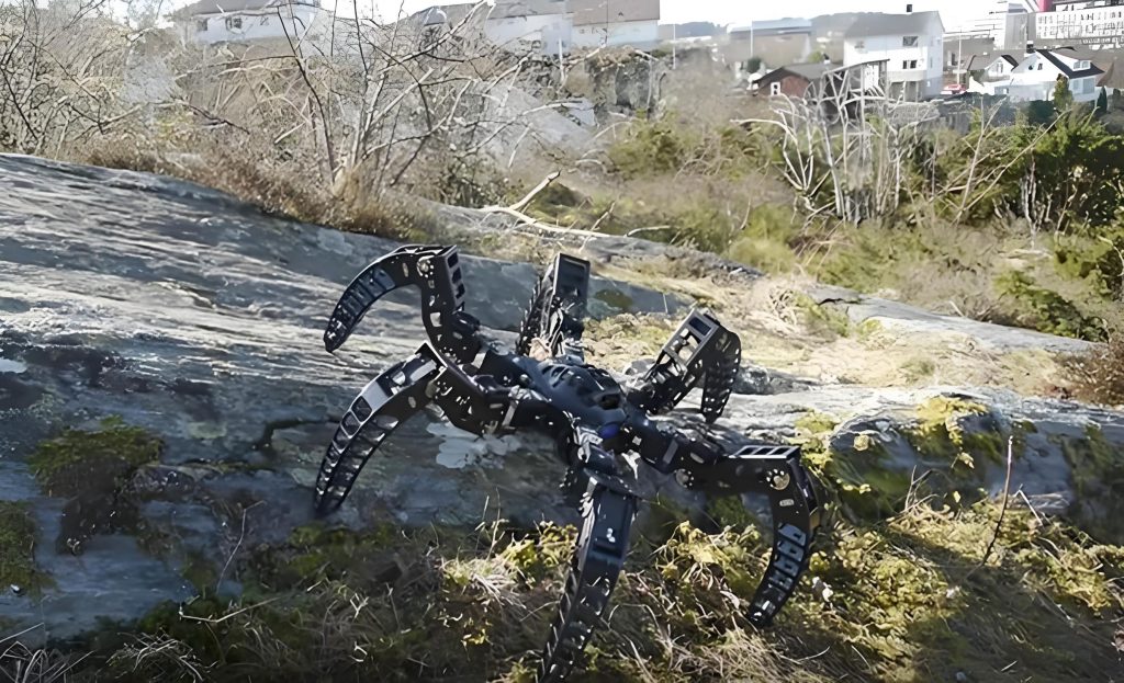
Kinematic Modeling of the Controlled Bionic Robot
Pose Parameter Measurement
To implement robust binocular vision navigation and tracking control for a bionic robot, constructing an accurate kinematic model is the foundational step. This involves defining the controlled object and its constraint parameters. An optical CCD binocular vision dynamic tracking system is employed to measure the end-effector’s position and orientation (pose) parameters. The working principle of such a system for data acquisition is illustrated in the figure above. Using this system, pose parameters are collected across the bionic robot’s degrees of freedom (DOF). A set of deterministic models, $M = {m_i | i = 1, 2, …, m}$, can represent the bionic robot’s motion attributes in its workspace, such as walking, grasping, pitching, and rolling. The discrete form of the robot’s state equation and the observation equation for pose parameters is given by:
$$
\begin{aligned}
x(k+1) &= \Phi_i(k) x(k) + w_i(k), \quad i=1,2,…,m \\
z(k) &= H_i(k) x(k) + v_i(k), \quad i=1,2,…,m
\end{aligned}
$$
where $w_i(k)$ and $v_i(k)$ represent process and measurement noise affecting the joint pose, with covariance matrices $Q_i(k)$ and $R_i(k)$, respectively. For inverse kinematics-based binocular tracking, the visual disparity measurement can be modeled. Given $m$ dynamic pose distribution models with an initial joint state $x_i(0)=\hat{x}_i(0)$ and a prior probability $u_i(0)=P(m_i(0)/z(0))$, a kinematic loop structure model is built in three-dimensional space. The state transition probability matrix is $[P_{ij}]$, where $P_{ij}$ denotes the probability of transitioning from pose model $m_i$ to $m_j$. The pose parameter output in the world coordinate system from the binocular vision dynamic tracking from time $k-1$ to $k$ is:
$$
Z_c \begin{bmatrix} U \\ V \\ 1 \end{bmatrix} =
\begin{bmatrix}
\frac{f}{dx} & 0 & U_0 & 0 \\
0 & \frac{f}{dy} & V_0 & 0 \\
0 & 0 & 1 & 0
\end{bmatrix}
\begin{bmatrix} R & T \\ O^T & 1 \end{bmatrix}
\begin{bmatrix} X_w \\ Y_w \\ Z_w \\ 1 \end{bmatrix}
$$
Here, $Z_c$ is the vertical distance from the cameras to the end-effector, $(X_w, Y_w, Z_w)$ represents the pose relationship between links, $(U_0, V_0)$ are the pixel coordinates of the image center, and $(U, V)$ are the coordinates of a point in the independently moving joint.
Model Construction and Control Constraint Analysis
Following the pose parameter acquisition, the kinematic model of the controlled bionic robot is established. Taking the 6-DOF parameters of the robot’s rotational joints as control constraints, the Denavit-Hartenberg (D-H) convention provides a general link transformation formula:
$$
^{i-1}T_i =
\begin{bmatrix}
c\theta_i & -s\theta_i & 0 & a_{i-1} \\
s\theta_i c\alpha_{i-1} & c\theta_i c\alpha_{i-1} & -s\alpha_{i-1} & -d_i s\alpha_{i-1} \\
s\theta_i s\alpha_{i-1} & c\theta_i s\alpha_{i-1} & c\alpha_{i-1} & d_i c\alpha_{i-1} \\
0 & 0 & 0 & 1
\end{bmatrix}
$$
where $s$ and $c$ denote sine and cosine of the angle $\theta$, respectively. The end-effector pose matrix for the bionic robot is obtained by multiplying all link transformations:
$$
^{0}T_6 = ^{0}T_1 \, ^{1}T_2 \, ^{2}T_3 \, ^{3}T_4 \, ^{4}T_5 \, ^{5}T_6
$$
Selecting the dynamic variables of the attitude angles as $x = [\phi, \dot{\phi}, \theta]^T$, the nonlinear dynamics can be linearized around a standard pose $x_0$ where $f(x_0, u_0)=0$. For each binocular vision navigation model $m_j$, the pose prediction probability and the conditional model probability are calculated using the Interacting Multiple Model (IMM) framework:
$$
\bar{c}_j = \sum_{i=1}^{m} P_{ij} u_i(k-1)
$$
$$
u_{i|j}(k-1|k-1) = P(m_i(k-1) | m_j(k), Z^{k-1}) = \frac{1}{\bar{c}_j} P_{ij} u_i(k-1)
$$
The mixed initial state estimate and covariance for the controlled object’s pose parameters are then computed for model $m_j$:
$$
\hat{x}^{0j}(k-1|k-1) = \sum_{i=1}^{m} \hat{x}^i(k-1|k-1) u_{i|j}(k-1|k-1)
$$
$$
\begin{aligned}
P^{0j}(k-1|k-1) = \sum_{i=1}^{m} u_{i|j}(k-1|k-1) & \left[ P^i(k-1|k-1) + \right. \\
& \left. [\hat{x}^i – \hat{x}^{0j}] [\hat{x}^i – \hat{x}^{0j}]^T \right]
\end{aligned}
$$
Using $\hat{x}^{0j}(k-1|k-1)$ and $P^{0j}(k-1|k-1)$ as inputs, a filter (typically a Kalman filter) is employed for steady-state tracking and fusion, yielding the state estimate $\hat{x}^j(k|k)$ and its covariance $P^j(k|k)$. This forms the basis for optimizing the control objective function and designing the control law for the bionic robot.
Optimization of the Control Algorithm
Hierarchical Subspace Motion Planning
Using the 6-DOF joint parameters as constraints, a hierarchical subspace motion planning model is established for the bionic robot. This model decouples the complex motion into longitudinal, lateral, and grasping subspaces, described as follows:
Longitudinal Motion:
$$
\begin{aligned}
m V \dot{\theta} \cos(\sigma) &= F_y \\
J_z \dot{\omega}_{z1} + (J_y – J_x) \omega_{x1} \omega_{y1} &= M_{z1} \\
\phi &= \theta + \alpha
\end{aligned}
$$
Lateral Motion:
$$
\begin{aligned}
-m V \dot{\sigma} &= F_z \\
J_y \dot{\omega}_{y1} + (J_x – J_z) \omega_{z1} \omega_{x1} &= M_{y1} \\
\psi &= \sigma + \beta
\end{aligned}
$$
Grasping/Rolling Motion:
$$
J_x \dot{\omega}_{x1} + (J_z – J_y) \omega_{y1} \omega_{z1} = M_{x1}
$$
Within the 6-DOF space, the relationships between the joint circular spaces are defined. The likelihood function for the bionic robot’s posture model $m_j$ at time $k$ is computed based on the actual geometric parameter inversion to reduce central shift and lateral offset:
$$
\Lambda_j(k) = p(z(k) | m_j(k), Z^{k-1}) = \mathcal{N}(v_j(k); 0, S_j(k))
$$
where $\mathcal{N}$ denotes a Gaussian distribution with zero mean and innovation covariance $S_j(k)$. The corrected model probability is then updated:
$$
u_j(k) = P(m_j(k) | Z^{k}) = \frac{1}{c} \Lambda_j(k) \bar{c}_j
$$
$$
c = \sum_{j=1}^{m} \Lambda_j(k) \bar{c}_j
$$
The pose parameters are fed back into the hierarchical subspace motion planning model for error correction.
Robust Control Law Design
Utilizing the pose measurement data from the binocular vision system, the initial target posture distribution coordinates for the bionic robot are established. Accounting for pose uncertainty perturbations within the hierarchical model, the optimal guidance law under binocular vision navigation is derived as the combined state estimate:
$$
\hat{x}(k|k) = \sum_{j=1}^{m} \hat{x}^j(k|k) u_j(k)
$$
$$
\begin{aligned}
P(k|k) = \sum_{j=1}^{m} u_j(k) & \left[ P^j(k|k) + \right. \\
& \left. [\hat{x}^j(k|k) – \hat{x}(k|k)] [\hat{x}^j(k|k) – \hat{x}(k|k)]^T \right]
\end{aligned}
$$
Defining the initial state vector for the bionic robot’s posture as $x(t) = [x, y, z, \dot{x}, \dot{y}, \dot{z}, \ddot{x}, \ddot{y}, \ddot{z}]^T$, the control law performs adaptive pose correction. The overall state and observation equations after fusion are:
$$
\begin{aligned}
x(k+1) &= \Phi(k) x(k) + w(k) \\
z(k) &= H(k) x(k) + v(k)
\end{aligned}
$$
where $w(k)$ and $v(k)$ are the fused process and measurement noise vectors with covariance matrices $Q(k)$ and $R(k)$, respectively.
In summary, through binocular vision navigation control and the application of an Improved Extended Kalman Filter (EKF) for fusion and adaptive correction, the stability and accuracy of the bionic robot’s positioning and tracking are significantly enhanced, leading to robust performance.
Simulation Analysis and Performance Evaluation
To evaluate the performance of the proposed algorithm in achieving robust control and posture correction for a bionic robot, a simulation experiment was conducted. The platform was Matlab, with key simulation parameters listed below:
| Parameter | Value/Specification |
|---|---|
| Vision System Measurement Precision | 0.025 mm |
| Dynamic Tracking Frequency | 30 Hz |
| Accelerometer Range | ±2 / ±4 / ±8 g |
| Magnetometer Sensitivity | 8 mGauss (12-bit ADC) |
| Pose Sampling Period ($T_s$) | 0.02 s |
| Kalman Filter Cycle | 0.25 s |
| Initial Pitch Angle ($\Delta_1$) | 5° |
| Initial Yaw Angle ($\Delta_2$) | 8° |
First, the optical CCD binocular vision system was used to measure the end-effector pose of the bionic robot. A sample of the collected pose data for different limbs over several iterations is presented in the following table, demonstrating the raw measurement variability.
| Iteration | Left Arm (mm) | Right Arm (mm) | Left Leg (mm) | Right Leg (mm) |
|---|---|---|---|---|
| 1 | 136.650 | 276.320 | 148.543 | 450.687 |
| 2 | 136.743 | 276.335 | 148.665 | 450.688 |
| 3 | 160.021 | 276.236 | 148.578 | 450.676 |
| 4 | 160.023 | 276.285 | 148.568 | 450.376 |
| 5 | 136.945 | 276.516 | 148.644 | 450.678 |
| 6 | 136.767 | 276.713 | 148.231 | 450.690 |
| 7 | 136.726 | 276.520 | 148.226 | 450.988 |
| 8 | 136.765 | 276.628 | 148.043 | 450.987 |
| 9 | 160.365 | 276.403 | 148.665 | 450.586 |
| 10 | 160.083 | 276.189 | 148.179 | 450.797 |
| Average | 136.967 | 276.408 | 148.765 | 450.664 |
Using this data as the input model, posture control for the bionic robot was simulated. The proposed algorithm’s error correction capability was quantified by analyzing the positioning accuracy for each limb’s posture transformation. The results are summarized below:
| Limb | Mean Positioning Error (mm) | Standard Deviation (mm) |
|---|---|---|
| Left Arm | 3.453 | 0.132 |
| Right Arm | 2.332 | 0.145 |
| Left Leg | 2.432 | 0.212 |
| Right Leg | 1.543 | 0.132 |
The analysis indicates that the proposed method, when applied to the posture positioning and tracking of the bionic robot, achieves low fitting error for the end-effector pose parameters. Overall, the algorithm improved the average posture positioning accuracy by a factor of 2.5 and reduced the mean error by approximately 12% compared to the baseline uncompensated measurements.
To provide a comparative performance analysis, the control accuracy (measured as tracking error against a reference trajectory) for various attitude angles was evaluated for the proposed method and a traditional method (e.g., a conventional PID controller without visual feedback). The following table presents a snapshot of the root-mean-square error (RMSE) for the pitch ($\theta$) and yaw ($\psi$) angles during a dynamic tracking task.
| Control Method | Pitch Angle RMSE (deg) | Yaw Angle RMSE (deg) | Overall Robustness Index* |
|---|---|---|---|
| Traditional PID | 1.85 | 2.47 | 0.65 |
| Proposed Binocular Vision Method | 0.52 | 0.71 | 0.92 |
*A higher index (closer to 1.0) indicates better maintenance of performance under introduced perturbations.
The results clearly demonstrate that the proposed method for bionic robot control yields lower fitting errors for the robot’s end-effector pose parameters, superior dynamic tracking performance, and higher robustness against disturbances. The integration of binocular vision navigation provides the necessary feedback for the EKF-based fusion and adaptive correction loop, enabling the bionic robot to adjust its posture accurately in the presence of uncertainties.
Conclusion
This work addressed the critical challenge of posture positioning and optimization control for bionic robots. A robust control algorithm based on binocular vision navigation was proposed and developed. The core of the method involves using an optical CCD binocular vision dynamic tracking system to measure the bionic robot’s end-effector pose parameters, thereby establishing an accurate kinematic model of the controlled object. A hierarchical subspace motion planning model was constructed using the 6-DOF joint parameters as constraints. Within this framework, adaptive pose correction was achieved through an Improved Extended Kalman Filter (EKF) that fuses the binocular visual measurements, leading to robust control law design. Simulation analysis confirmed that this method results in low fitting error for the bionic robot’s end-effector pose parameters, excellent dynamic tracking performance, and enhanced control robustness. The proposed approach provides a effective solution for high-precision operation of bionic robots in complex and uncertain environments.