
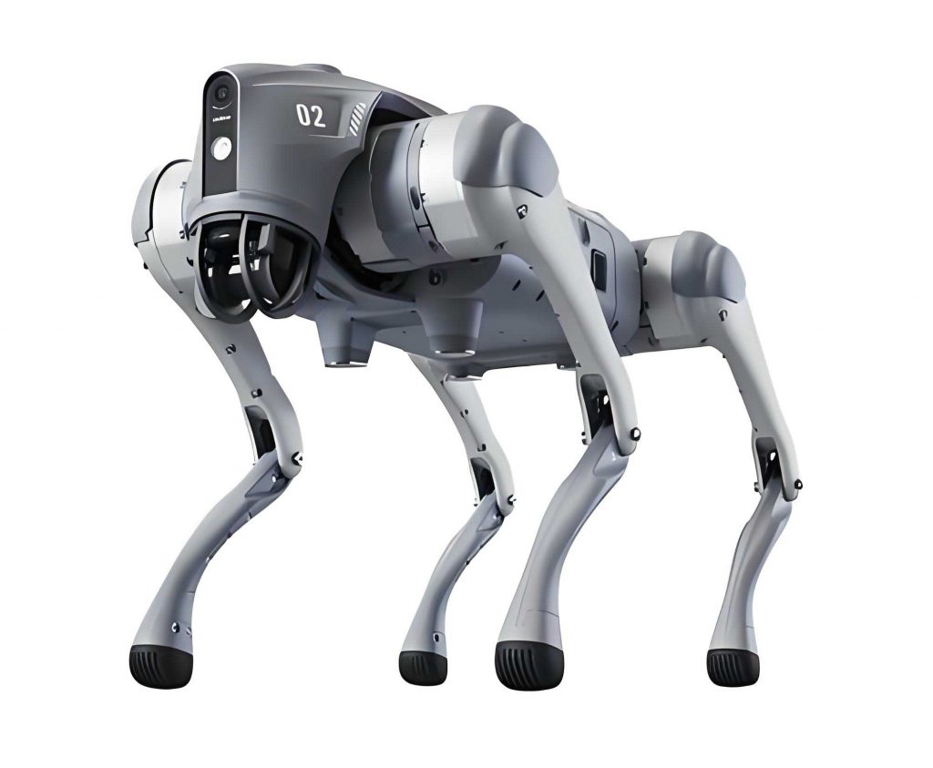
In recent years, the field of mobile robotics has seen significant advancements in biomimetic legged systems, with the quadruped robot emerging as a prominent focus due to its superior mobility, agility, and adaptability across diverse terrains. As a researcher engaged in this domain, I have observed that while legged robots can achieve basic locomotion through kinematic trajectory planning, issues such as foot slippage, inconsistent foot-end velocities, and directional instability during gait cycles often compromise overall system performance. Relying solely on kinematic models for position and trajectory control proves insufficient for ensuring robust stability, particularly in dynamic environments. To address these challenges, my work explores the application of Virtual Model Control (VMC), a method that simplifies the complex dynamics of quadruped robots by leveraging virtual components to generate control forces and torques. This approach transforms high-level posture and velocity commands into joint-level torque instructions, enabling holistic control of the robot’s body. Through extensive simulation and analysis, I investigate how parameters like damping and stiffness coefficients influence foot-end trajectories, yaw displacement, and center-of-mass height, ultimately demonstrating that VMC significantly enhances directional stability and walking robustness for quadruped robots.
The core principle of Virtual Model Control lies in its use of imaginary mechanical elements, such as springs and dampers, to create virtual forces and torques that guide the robot’s motion without physical implementation. For a quadruped robot, this involves defining these virtual components between the robot’s feet and the environment, allowing for a simplified representation of the system’s dynamics. The relationship between foot-end forces and joint torques is derived through the robot’s kinematics. Let the foot-end position in Cartesian space be represented as \( \mathbf{x} = [x_1, x_2, \dots, x_n]^T \), and the joint angles as \( \mathbf{q} = [q_1, q_2, \dots, q_m]^T \). The forward kinematics equation is given by \( \mathbf{x} = f(\mathbf{q}) \). By differentiating this, we obtain the Jacobian matrix \( \mathbf{J} \), which maps joint velocities to foot-end velocities:
$$ \delta \mathbf{x} = \mathbf{J} \cdot \delta \mathbf{q}, $$
where \( \mathbf{J} \) is defined as:
$$ \mathbf{J} = \begin{bmatrix} \frac{\partial f_1}{\partial q_1} & \cdots & \frac{\partial f_1}{\partial q_m} \\ \vdots & \ddots & \vdots \\ \frac{\partial f_n}{\partial q_1} & \cdots & \frac{\partial f_n}{\partial q_m} \end{bmatrix}. $$
Applying the principle of virtual work, which states that the total virtual work done by all forces is zero, we derive the relationship between joint torques \( \boldsymbol{\tau} \) and external forces \( \mathbf{F} \):
$$ \boldsymbol{\tau}^T \delta \mathbf{q} + (-\mathbf{F})^T \delta \mathbf{x} = 0 \quad \Rightarrow \quad \boldsymbol{\tau} = \mathbf{J}^T \mathbf{F}. $$
This equation forms the foundation of VMC, as it allows us to compute the required joint torques based on virtual forces generated by spring-damper systems. For instance, the virtual force \( \mathbf{F}_u \) in a direction \( u \) can be expressed as:
$$ F_u = B (\dot{u}_d – \dot{u}) + K (u_d – u), $$
where \( B \) is the damping coefficient, \( K \) is the stiffness coefficient, \( u_d \) and \( \dot{u}_d \) are the desired position and velocity, and \( u \) and \( \dot{u} \) are the actual values. This formulation enables precise control of the quadruped robot’s foot-end trajectories during both support and swing phases, ensuring stable interaction with the ground.
In implementing VMC for a quadruped robot’s leg control, we focus on the kinematic model of each limb. For example, consider the right front leg of a robot dog, where the foot-end position relative to the hip joint is derived from the joint angles. Let \( \theta_1 \), \( \theta_2 \), and \( \theta_3 \) represent the abduction, hip, and knee joint angles, respectively, with link lengths \( L_1 \), \( L_2 \), and \( L_3 \). The foot-end coordinates \( [P_x, P_y, P_z]^T \) are given by:
$$ \begin{aligned} P_x &= L_2 \cos \theta_1 \cos \theta_2 + L_3 \cos \theta_1 \cos (\theta_2 + \theta_3) – L_1 \sin \theta_1, \\ P_y &= L_2 \sin \theta_1 \cos \theta_2 + L_3 \sin \theta_1 \cos (\theta_2 + \theta_3) + L_1 \cos \theta_1, \\ P_z &= -L_3 \sin (\theta_2 + \theta_3) – L_2 \sin \theta_2. \end{aligned} $$
The Jacobian matrix for this leg, \( \mathbf{J}_{\text{RF}} \), is computed by partial differentiation of these equations with respect to the joint angles. For control purposes, virtual forces are applied in the x, y, and z directions. During the support phase, the virtual force \( \mathbf{F}_{\text{RF}} \) is designed to maintain body support and propulsion:
$$ \mathbf{F}_{\text{RF}} = \begin{bmatrix} f_x \\ f_y \\ f_z \end{bmatrix} = \begin{bmatrix} 0 \\ 0 \\ K_z \end{bmatrix} (z_d – z) + \begin{bmatrix} B_x \\ B_y \\ B_z \end{bmatrix} \begin{bmatrix} \dot{x}_d – \dot{x} \\ \dot{y}_d – \dot{y} \\ \dot{z}_d – \dot{z} \end{bmatrix}, $$
where \( K_z \) and \( B_z \) are the stiffness and damping coefficients in the vertical direction, and subscript \( d \) denotes desired values. In contrast, during the swing phase, the virtual force includes positional feedback in all directions to track the planned trajectory:
$$ \mathbf{F}_{\text{RF}} = \begin{bmatrix} K_x & 0 & 0 \\ 0 & K_y & 0 \\ 0 & 0 & K_z \end{bmatrix} \begin{bmatrix} x_d – x \\ y_d – y \\ z_d – z \end{bmatrix} + \begin{bmatrix} B_x & 0 & 0 \\ 0 & B_y & 0 \\ 0 & 0 & B_z \end{bmatrix} \begin{bmatrix} \dot{x}_d – \dot{x} \\ \dot{y}_d – \dot{y} \\ \dot{z}_d – \dot{z} \end{bmatrix}. $$
These virtual forces are then transformed into joint torques using \( \boldsymbol{\tau} = \mathbf{J}^T \mathbf{F} \), enabling real-time control of the quadruped robot’s legs. The following table summarizes the virtual force components for different phases:
| Phase | Virtual Force Components | Description |
|---|---|---|
| Support | \( f_x = B_x (\dot{x}_d – \dot{x}) \), \( f_y = B_y (\dot{y}_d – \dot{y}) \), \( f_z = K_z (z_d – z) + B_z (\dot{z}_d – \dot{z}) \) | Focus on vertical support and damping |
| Swing | \( f_i = K_i (i_d – i) + B_i (\dot{i}_d – \dot{i}) \) for \( i = x, y, z \) | Full positional and velocity tracking |
Directional control is critical for the quadruped robot to navigate complex environments. The yaw angle \( \psi \), representing the robot’s heading, is controlled by applying a virtual torque around the z-axis. This torque \( M_\psi \) is generated based on the error between the desired and actual yaw angles and angular velocities:
$$ M_\psi = K_\psi (\psi_d – \psi) + B_\psi (\dot{\psi}_d – \dot{\psi}), $$
where \( K_\psi \) and \( B_\psi \) are the yaw stiffness and damping coefficients. To realize this torque, differential lateral forces are applied to the supporting legs. For instance, if the robot needs to turn clockwise, the left supporting legs exert a forward lateral force while the right legs exert a backward force, creating a net torque. The lateral force adjustment \( \Delta f_y \) for each supporting leg is computed as:
$$ \Delta f_y = \frac{K_\psi (\psi_d – \psi) + B_\psi (\dot{\psi}_d – \dot{\psi})}{W}, $$
where \( W \) is the lateral distance from the center of mass to the foot contact point. This ensures that the total lateral force remains balanced, preventing unwanted side-slipping. The modified virtual force for a supporting leg during turning becomes:
$$ \mathbf{F}’ = \begin{bmatrix} f_x \\ f_y + \Delta f_y \\ f_z \end{bmatrix}. $$
To prevent excessive joint angles and instability, the yaw rate \( \dot{\psi} \) is constrained within limits \( \dot{\psi}_{\text{min}} \leq \dot{\psi} \leq \dot{\psi}_{\text{max}} \). This approach allows the quadruped robot to achieve smooth and stable turning motions while maintaining overall balance.
In simulation experiments, we evaluated the performance of the VMC framework for a quadruped robot using MATLAB/Simulink. The robot model had a body height of 0.35 m, and the gait cycle period was set to 0.5 s with a step length of 0.22 m and a leg lift height of 0.13 m. The initial body orientation was zero for yaw, pitch, and roll angles. We analyzed the effects of damping and stiffness coefficients on foot-end trajectories, yaw displacement, and center-of-mass height. For the damping coefficient \( B \), we tested values from 50 to 250 N·s/m while keeping the stiffness \( K \) constant at 2000 N/m. The results showed that lower damping led to significant oscillations and yaw deviation, whereas higher damping reduced amplitude but introduced tracking errors in the foot-end path. The following table outlines the impact of varying \( B \) on key metrics:
| Damping Coefficient \( B \) (N·s/m) | Foot-End Trajectory Error | Yaw Displacement | Center-of-Mass Stability |
|---|---|---|---|
| 50 | High oscillation, poor tracking | Large deviation | Unstable |
| 100 | Moderate error | Reduced yaw | Improved |
| 150 | Low oscillation | Minor deviation | Stable |
| 200 | Smooth but offset | Minimal | Very stable |
| 250 | High offset from desired | Negligible | Over-damped |
For the stiffness coefficient \( K \), we varied it from 800 to 3200 N/m with a fixed damping of 100 N·s/m. Higher stiffness improved trajectory tracking but increased sensitivity to disturbances, while lower stiffness resulted in sluggish response and greater foot slippage. The optimal values were identified as \( K_x = 3200 \) N/m, \( K_y = 1400 \) N/m, \( K_z = 3200 \) N/m, and \( B_x = 70 \) N·s/m, \( B_y = 100 \) N·s/m, \( B_z = 70 \) N·s/m. These settings minimized yaw error and ensured smooth foot-end trajectories for the quadruped robot. The virtual forces and torques were computed in real-time, and the joint torques were derived using the Jacobian transpose method. For example, the joint torques \( \boldsymbol{\tau} \) for a leg are given by:
$$ \boldsymbol{\tau} = \mathbf{J}^T \mathbf{F}, $$
where \( \mathbf{F} \) is the virtual force vector. In turning scenarios, the yaw control demonstrated effective tracking of desired headings, such as a sequence of step changes in \( \psi_d \): 0.2 rad for 0-20 s, 0.785 rad for 20-40 s, 1.57 rad for 40-60 s, and 0.785 rad for 60-80 s. With yaw rate constraints of \( -0.5 \leq \dot{\psi} \leq 0.5 \) rad/s, the robot dog maintained stability without exceeding joint limits. The lateral swing joint torques varied symmetrically during turns, while hip and knee joints provided propulsion and support. The center-of-mass height remained within 0.34-0.36 m, indicating minimal pitch and roll oscillations.
In conclusion, the Virtual Model Control approach offers a robust framework for stable walking control of quadruped robots. By leveraging virtual spring-damper systems, we simplify the complex dynamics of a robot dog and achieve precise joint-level torque control. The selection of appropriate stiffness and damping coefficients is crucial for balancing trajectory tracking and stability. Through simulation, we have shown that VMC effectively reduces yaw displacement, improves foot-end trajectory accuracy, and enhances overall directional stability. This method proves particularly advantageous for quadruped robots operating in dynamic environments, where adaptability and robustness are paramount. Future work will focus on extending VMC to handle uneven terrains and integrating sensor feedback for real-time parameter adjustment.