
The pursuit of reliability in robotic systems places immense importance on the core transmission components. Among these, the rotary vector reducer stands out due to its compact structure, high torque capacity, and superior precision, making it a cornerstone in industrial robot joints. Consequently, the condition monitoring and fault diagnosis of the rotary vector reducer are critical for ensuring the operational safety and longevity of the entire robotic system. While data-driven artificial intelligence (AI) methods have shown remarkable promise in this domain, their deployment in practical engineering is fundamentally constrained by a pervasive challenge: the scarcity of physical fault samples. It is impractical and costly to run critical components like a rotary vector reducer to failure repeatedly to collect comprehensive fault data. This data paucity severely limits the generalization ability and diagnostic accuracy of AI models trained solely on limited, often idealized, experimental data.
To address this foundational limitation, this article proposes a novel methodology that shifts the paradigm from being purely data-driven to being dynamic model-driven. The core idea is to leverage high-fidelity dynamic simulations of the rotary vector reducer to generate a vast, customizable library of fault vibration data. This synthetically generated data can then be used to train robust AI diagnostic models, effectively solving the problem of fault sample insufficiency. The process involves several key steps: first, establishing and meticulously refining a high-precision dynamic model of a healthy rotary vector reducer; second, integrating mathematically formulated fault models (e.g., gear wear, crack, breakage) into this baseline model to simulate faulty conditions; third, using the simulated vibration signals as abundant training samples for an AI classifier; and finally, validating the trained model’s ability to diagnose real-world, unknown faults collected from a physical test rig.
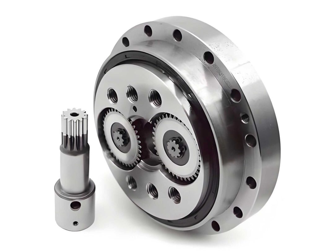
The rotary vector reducer is a complex two-stage transmission system. The first stage is a planetary gear train, and the second stage is a cycloid-pin gear mechanism. Constructing an accurate dynamic model requires accounting for these interconnected subsystems. Using the lumped-parameter method, a 26-degree-of-freedom (DOF) translational-torsional coupled dynamic model is developed. This model encompasses key components: the sun gear (input), planets, crankshafts, cycloid gears, and the output disk. The model incorporates essential nonlinear factors such as time-varying mesh stiffness (TVMS) for all gear pairs, bearing support stiffness and damping, and gear backlash. The following assumptions are made to render the model tractable while retaining critical dynamics: all identical components have uniform parameters; gyroscopic effects are negligible; the input speed is constant; and influences of gravity and friction are excluded.
The establishment of the equations of motion is performed in rotating coordinate systems to simplify the expression of relative displacements. For components rotating with the output carrier (sun gear, output disk), a central member coordinate system is used. For components that orbit the center (planets, crankshafts, cycloids), a planetary member coordinate system is employed. The absolute accelerations in these rotating frames include Coriolis and centrifugal terms. The kinetic energy (T), potential energy (U), and dissipation function (D) of the entire system are formulated based on the defined coordinates and relative displacements. Applying Lagrange’s equation yields the complete set of nonlinear differential equations governing the system’s motion.
To illustrate the model’s structure, the parameters for a representative rotary vector reducer model are summarized in the table below.
| Component | Mass (kg) | Moment of Inertia (kg·m²) | Radius (m) |
|---|---|---|---|
| Sun Gear | 0.190 | 1.66e-5 | 6.3e-3 |
| Planet Gear | 0.0492 | 9.84e-6 | 1.9e-2 |
| Crankshaft | 0.0576 | 1.04e-6 | 2.2e-3 |
| Cycloid Gear | 0.5203 | 6.18e-4 | 4.8e-2 |
| Output Disk | 2.9 | 3.8e-3 | 5.2e-2 |
The relative displacement between the sun gear and a planet gear along the line of action, considering backlash, is a key driver of vibration. It can be expressed as:
$$ \delta_{si} = x_s \cos\phi_{si} + y_s \sin\phi_{si} + r_s \theta_s – x_{pi} \sin\alpha_s – y_{pi} \cos\alpha_s – r_p \theta_{pi} $$
where $\phi_{si} = \psi_i + \alpha_s$, $\alpha_s$ is the pressure angle, and $\psi_i$ is the planet’s angular position. The nonlinear backlash function $f(\delta_{si}, b)$ is applied to this displacement.
A critical step in making the simulation useful for real-world diagnosis is model updating. Initial simulation results from a purely theoretical model will inevitably deviate from actual measured vibrations due to unmodeled dynamics and parameter uncertainties. To bridge this gap, a similarity metric is used to calibrate the model. The Pearson Correlation Coefficient (PCC) is chosen for its effectiveness in measuring linear correlation and scale invariance. The PCC $r$ between a simulated signal $X$ and a measured signal $Y$ is:
$$ r = \frac{\sum_{i=1}^{n} (X_i – \bar{X})(Y_i – \bar{Y})}{\sqrt{\sum_{i=1}^{n} (X_i – \bar{X})^2 \sum_{i=1}^{n} (Y_i – \bar{Y})^2}} $$
Model parameters (e.g., stiffness, damping) are iteratively adjusted until the PCC between the healthy model’s output and a baseline experimental measurement exceeds a threshold (e.g., 0.7), ensuring the dynamic model possesses a satisfactory level of fidelity.
The internal excitation from gear mesh stiffness is paramount, especially when simulating faults. The time-varying mesh stiffness (TVMS) for healthy gears is calculated using the potential energy method, considering Hertzian contact stiffness $k_h$, bending stiffness $k_b$, shear stiffness $k_s$, and axial compressive stiffness $k_a$. The total mesh stiffness for a sun-planet pair is a combination of these:
$$ \frac{1}{k_{sp}} = \frac{1}{k_h} + \frac{1}{k_{b1}} + \frac{1}{k_{b2}} + \frac{1}{k_{s1}} + \frac{1}{k_{s2}} + \frac{1}{k_{a1}} + \frac{1}{k_{a2}} + \frac{1}{k_{f1}} + \frac{1}{k_{f2}} $$
where subscripts 1 and 2 denote the sun and planet, respectively. For dual-tooth contact phases, the stiffnesses are summed in parallel.
To simulate faults, mathematical models of degraded gear teeth are integrated into the TVMS calculation. For wear, the Archard wear model informs a non-uniform wear depth $h_w$ along the tooth profile. This wear depth modifies the effective tooth thickness $h_x$ and the area $A_x$ and moment of inertia $I_x$ of the tooth cross-section used in the stiffness calculations:
$$ h_x’ = h_x – h_w \cos\alpha $$
$$ A_x’ = (h_x’ ) L $$
$$ I_x’ = \frac{1}{12} (h_x’ )^3 L $$
These modified geometric parameters lead to a reduction in $k_b$, $k_s$, and $k_a$, thereby lowering the overall TVMS, as shown in simulation results.
For crack faults, the crack propagation path is modeled, leading to a reduction in the effective area and moment of inertia of the tooth root section. The calculation is segmented into different cases depending on whether the crack has passed the tooth centerline. The formulas for $A_x$ and $I_x$ are piecewise, incorporating crack length $q$ and angle $v$. For a crack before passing the centerline (Case 1, where $h_a \ge h_0$ and $\alpha_1 > \alpha_a$):
$$ I_x = \begin{cases} \frac{1}{12}(h_a + h_x)^3 L & x > d_a \\ \frac{1}{12}(2h_x)^3 L & x \le d_a \end{cases} $$
These modifications result in a characteristic, localized reduction in the TVMS waveform at the cracked tooth’s engagement position.
For a broken tooth, the model is straightforward: during the meshing period of the broken tooth, the mesh stiffness contribution for that tooth pair is set to zero. In double-tooth contact, this means only one pair carries the load; in single-tooth contact, it implies a complete loss of mesh stiffness for that interval, causing a significant impulse in the dynamic response.
With the updated healthy model and the fault-modulated TVMS models, the nonlinear differential equations are solved numerically (e.g., using Runge-Kutta methods) to generate vibration acceleration signals. For this study, six distinct health states are simulated: T1 (Healthy), T2 (Tooth Break), T3 (Wear), T4 (Crack), T5 (Break+Wear), T6 (Break+Wear+Crack). To make the synthetic data more realistic and improve the AI model’s robustness, additive white Gaussian noise (AWGN) is injected into the signals:
$$ \text{Data}_{\text{Noise}} = \text{awgn}(\text{Data}_{\text{Pure}}, \text{SNR}) $$
A long-duration simulation (e.g., 60 seconds at 48 kHz) is performed for each state. This long signal is then segmented into numerous short samples (e.g., 8000 data points each), creating a large, balanced dataset for AI training. For instance, 260 samples per fault class can be used for training and 100 for testing the AI model internally.
The Convolutional Neural Network (CNN) is selected as the intelligent classifier due to its strong capability in automatically learning discriminative features from raw vibration data. A 1D-CNN architecture is suitable for temporal signals. The simulated fault samples from all six states form the training set. The CNN model typically includes consecutive layers of 1D convolution, activation functions (ReLU), pooling layers for dimensionality reduction, followed by flattening and fully connected layers leading to a final softmax output for 6-class classification. The training process minimizes a cross-entropy loss function, enabling the network to learn the unique patterns associated with each fault type from the simulation data alone.
The ultimate test of this dynamic model-driven approach is its performance on real-world data. An experimental test rig for a rotary vector reducer is set up, incorporating motors, loads, and accelerometers. Vibration data is collected for various induced fault conditions (e.g., worn gear, cracked gear). Crucially, this experimental data is completely unseen by the CNN model during training; it serves exclusively as the final validation set. The experimental signals are preprocessed identically to the training data (segmented into samples) and fed into the trained CNN for classification.
The results demonstrate the efficacy of the method. The CNN, trained solely on data generated from the dynamic model of the rotary vector reducer, successfully identifies the actual faults from the experimental measurements with high accuracy. Multiple trials yield consistent results, confirming the model’s robustness. The classification accuracy for different fault types is summarized below:
| Fault Type | Label | Best Accuracy (%) | Average Accuracy (%) |
|---|---|---|---|
| Healthy (T1) | 1 | 100 | 99.2 |
| Break (T2) | 2 | 100 | 99.6 |
| Wear (T3) | 3 | 100 | 98.8 |
| Crack (T4) | 4 | 100 | 99.6 |
| Break+Wear (T5) | 5 | 100 | 100 |
| Break+Wear+Crack (T6) | 6 | 100 | 99.2 |
In conclusion, this work presents a practical and powerful solution to a fundamental bottleneck in AI-based fault diagnosis for critical components like the rotary vector reducer. By shifting the source of training data from scarce physical experiments to high-fidelity dynamic simulations, the method circumvents the problem of fault sample insufficiency. The process involves constructing and refining a precise dynamic model, integrating physics-based fault models, generating a comprehensive synthetic dataset, and training an AI diagnostic model. The successful application of a CNN model trained on simulated data to diagnose real faults in a rotary vector reducer validates the entire pipeline. This dynamic model-driven intelligent diagnosis framework is not limited to rotary vector reducers but can be extended to other complex mechanical systems, offering a generalizable strategy for developing reliable, data-efficient condition monitoring solutions where failure data is naturally scarce. The synergy between high-precision modeling and modern AI unlocks a path toward more robust and accessible predictive maintenance for advanced machinery.