
The precision of rotary vector (RV) reducers is paramount in applications such as industrial robotic joints, where high transmission accuracy, compact structure, and robustness are critical. As a core component, the RV reducer combines a primary planetary gear stage with a secondary cycloidal-pin gear stage, offering superior load capacity and efficiency. However, the transmission precision of the RV reducer is inherently influenced by various deviations arising from part manufacturing and assembly processes. This study delves into the propagation of these deviations under static assembly conditions, employing a directed graph approach to model and analyze the intricate relationships between part errors. The objective is to establish a clear framework for understanding how deviations accumulate and affect the overall kinematic accuracy of the RV reducer system.
Deviations in mechanical assemblies are inevitable due to tolerances in manufacturing and uncertainties in assembly. For the RV reducer, these deviations can be systematically categorized into three primary sources, each contributing uniquely to the final output error. The first category, geometric position deviations (denoted as \(E_1\)), encompasses errors related to the location and orientation of part features. This includes dimensional tolerances (e.g., diameter variations), coaxiality errors between axes, parallelism, and perpendicularity deviations. For instance, the coaxiality error between the input shaft and the sun gear axis, or the parallelism error between the input shaft and the crank shaft axes, falls under \(E_1\). The second category, geometric form deviations (\(E_2\)), relates to the shape imperfections of part surfaces, such as cylindricity, circularity, straightness, and profile errors. An example is the cycloidal profile error on the cycloidal gear. The third category, assembly position deviations (\(E_3\)), arises during the assembly process itself. This includes errors due to fixturing, locating inaccuracies, and the inherent play or clearance in fits, which can cause parts to assume uncertain positions relative to their nominal locations. These three deviation sources often couple nonlinearly, ultimately degrading the transmission precision of the RV reducer.
To model the propagation of these deviations through the assembly, we introduce the concept of a deviation directed graph. This graph-based representation captures how errors transfer from one component to another via mating interfaces. Two fundamental propagation mechanisms are identified. The first, denoted \(H_a\), is geometric deviation propagation. When two parts mate, their individual deviations (both \(E_1\) and \(E_2\)) interact, causing a shift in the relative pose of the parts. This shifted pose then becomes a new deviation input for subsequent assemblies, leading to cumulative error build-up along a chain of components. The second mechanism, \(H_b\), is assembly position deviation propagation. This occurs specifically at interfaces with clearance fits. Here, the deviation accumulation from upstream parts may be “reset” or isolated; the downstream part’s position is primarily governed by its own local deviations and the clearance, causing a discontinuity in the error propagation path. Understanding the interplay between \(H_a\) and \(H_b\) is crucial for accurate error budgeting in the RV reducer.
The directed graph model formalizes these concepts. Each part is represented by nodes corresponding to its geometric features (e.g., axes, surfaces). Deviation sources \(E_1\), \(E_2\), and \(E_3\) are modeled as directed edges or inputs to these geometric nodes. The mating relationships between parts, such as shaft-hole fits or gear meshes (treated as surface-surface contacts), are represented as special nodes that combine deviations from both mating parts. A basic deviation flow model can be expressed using a set of equations. Let \(g_{ij}\) represent the \(j\)-th geometric element of part \(i\), and \(d_x\) represent a deviation source. The influence of a deviation on a geometric element can be modeled as a transformation. For a simple linear stack-up, the resultant error \(\Delta g\) on a feature due to multiple deviations can be approximated as a sum:
$$\Delta g = \sum_{k} \mathbf{J}_{k} \cdot d_{k}$$
where \(\mathbf{J}_{k}\) is the Jacobian matrix representing the sensitivity of the geometric feature to the \(k\)-th deviation source \(d_{k}\). In the context of the RV reducer, these deviations include dimensional errors and misalignments. For the directed graph, we define four fundamental deviation flow patterns, as illustrated conceptually. For example, the coupling of an assembly position deviation \(d_{13}\) (from part 1) with other deviations \(d_0\) affecting the geometric feature \(g_{21}\) of part 2 can be represented as a node where edges \(d_0\) and \(d_{13}\) converge onto \(g_{21}\).
Mating conditions are critical nodes in the graph. A shaft-hole fit involves two geometric elements: the shaft cylinder (e.g., \(g_{10}\)) and the hole cylinder (e.g., \(g_{20}\)). The resultant fit deviation \(d_0\) is a function of the individual deviations of both the shaft and the hole, which themselves are influenced by the deviations of their parent parts. Similarly, a surface-surface contact (like gear teeth meshing) involves two planar or curved surfaces. The directed graph model for a mating condition \(m\) is shown below, where \(g_{1i}\) and \(g_{2j}\) are the mating geometries from parts 1 and 2, respectively, and \(d_{1i}\) to \(d_{2j}\) are the deviation sources affecting those geometries.
| Mating Type | Geometry from Part 1 | Geometry from Part 2 | Key Deviation Sources | Propagation Type |
|---|---|---|---|---|
| Shaft-Hole Fit | Shaft axis/surface \(g_{1a}\) | Hole axis/surface \(g_{2a}\) | Diameter tol., coaxiality (\(E_1\)), cylindricity (\(E_2\)) | Mostly \(H_a\) (if interference/transition), can involve \(H_b\) (if clearance) |
| Surface-Surface Contact | Gear tooth flank \(g_{1b}\) | Gear tooth flank \(g_{2b}\) | Profile error (\(E_2\)), pitch error, alignment (\(E_1\)) | Primarily \(H_a\) |
| Bearing Mounting | Bore surface \(g_{1c}\) | Bearing OD \(g_{2c}\) | Diameter tol., roundness (\(E_2\)), assembly shift (\(E_3\)) | Combination of \(H_a\) and \(H_b\) |
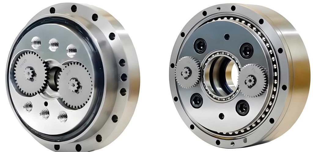
The power of the directed graph approach is demonstrated through a detailed case study of an RV320S-type reducer. The RV reducer assembly consists of multiple components: input shaft, sun gear, planetary gears, crank shafts, bearings, cycloidal gears, pin sleeves, pin shafts, and the output plate. Each component carries its own set of potential deviations as per the three categories. The tables below comprehensively list the deviation types for each part and the mating conditions between them.
| Component | Geometric Position Deviations (\(E_1\)) | Geometric Form Deviations (\(E_2\)) | Assembly Position Deviations (\(E_3\)) |
|---|---|---|---|
| Input Shaft | Diameter tolerance; Coaxiality error w.r.t. sun gear axis | Cylindricity; Circular run-out | Fit deviation in sun gear bore |
| Sun Gear | Diameter tolerance; Coaxiality error; Parallelism/Perpendicularity of faces | Tooth profile error | Fit deviation with input shaft; Mesh deviation with planet gears |
| Planet Gear | Diameter tolerance; Coaxiality error w.r.t. crank shaft; Face orientation errors | Tooth profile error | Fit deviation on crank shaft; Mesh deviation with sun gear |
| Crank Shaft | Diameter tolerance; Coaxiality error w.r.t. input shaft axis | Cylindricity; Circular run-out | Fit deviations for planet gear and bearings |
| Cycloidal Gear | Diameter tolerance; Coaxiality error w.r.t. crank shaft; Face orientation errors | Cycloidal profile error; Surface waviness | Clearance fit deviations with bearing assemblies |
| Bearing I/II | Coaxiality error w.r.t. mating shaft/housing | Raceway roundness; Ball geometry errors | Radial/axial play; Mounting misalignment |
| Pin Sleeve & Pin | Diameter tolerance; Coaxiality between sleeve and pin | Cylindricity; Roundness | Fit deviation between sleeve and pin; Contact deviation with cycloid gear |
| Output Plate | Diameter tolerance; Coaxiality w.r.t. input and crank shafts | Face flatness; Bore cylindricity | Fit deviation with bearing |
| Mating Pair | Mating Type (Symbol) | Geometry 1 (Part) | Geometry 2 (Part) | Critical Deviation Parameters |
|---|---|---|---|---|
| Input Shaft – Sun Gear | Shaft-hole fit (\(m_1\)) | Shaft journal \(g_{11}\) (Input) | Bore \(g_{21}\) (Sun Gear) | \(\delta D_{in}\), \(\delta D_{sun}\), coaxiality \(\phi_{11}\) |
| Sun Gear – Planet Gear | Gear mesh (\(m_2\)) | Tooth flank \(g_{22}\) (Sun) | Tooth flank \(g_{32}\) (Planet) | Profile errors \(\Delta p_{22}, \Delta p_{32}\); Center distance variation |
| Planet Gear – Crank Shaft | Shaft-hole fit (\(m_3\)) | Bore \(g_{31}\) (Planet) | Journal \(g_{41}\) (Crank) | \(\delta D_{plan}\), \(\delta D_{crank}\), hole position error |
| Crank Shaft – Bearing I | Shaft-hole fit (\(m_4\)) | Journal \(g_{41}\) (Crank) | Inner race bore \(g_{51}\) (Bearing I) | \(\delta D_{crank}\), \(\delta D_{bearing}\), mounting squareness |
| Bearing I – Cycloid Gear | Clearance fit (\(m_5\)) | Outer race O.D. \(g_{52}\) (Bearing I) | Bore \(g_{61}\) (Cycloid Gear) | Radial clearance \(C_r\), bore diameter error \(\delta D_{cycl}\) |
| Cycloid Gear – Pin Sleeve | Surface contact (\(m_6\)) | Cycloid tooth flank \(g_{62}\) (Cycloid) | Outer surface \(g_{72}\) (Pin Sleeve) | Cycloid profile error \(\Delta c_{62}\), pin circle radius error |
| Pin Sleeve – Pin | Shaft-hole fit (\(m_7\)) | Bore \(g_{71}\) (Sleeve) | Pin diameter \(g_{81}\) (Pin) | \(\delta D_{sleeve}\), \(\delta D_{pin}\), pin position tolerance |
| Cycloid Gear – Bearing II | Clearance fit (\(m_8\)) | Bore \(g_{63}\) (Cycloid) | Outer race O.D. \(g_{92}\) (Bearing II) | Radial clearance, axial play, bore form error |
| Bearing II – Output Plate | Shaft-hole fit (\(m_9\)) | Inner race bore \(g_{91}\) (Bearing II) | Bore \(g_{101}\) (Output Plate) | \(\delta D_{bearing2}\), \(\delta D_{out}\), fit interference variation |
The assembly position requirements, which define the functional relationships between key axes, are equally important for establishing the deviation propagation paths. These requirements, such as the coaxiality of the output shaft relative to the input shaft, serve as global constraints in the directed graph. The error in fulfilling these requirements is the ultimate measure of transmission inaccuracy. For the RV320S reducer, we define a set of critical axis relationships, where \(g_{i0}\) denotes the axis of part \(i\), and \(E_{ij0}\) represents the deviation of axis \(i\) relative to axis \(j\). For instance, \(E_{1010}\) is the output axis deviation relative to the input axis, which directly impacts the RV reducer’s angular transmission error.
| Position Requirement Description | Functional Geometry (\(g_{i0}\)) | Reference Geometry (\(g_{j0}\)) | Resultant Deviation Symbol | Sensitivity Coefficient (Approx.) |
|---|---|---|---|---|
| Sun gear axis relative to input axis | \(g_{20}\) (Sun) | \(g_{10}\) (Input) | \(E_{210}\) | \(J_{21}\) (from fit \(m_1\)) |
| Planet gear axis relative to sun gear axis | \(g_{30}\) (Planet) | \(g_{20}\) (Sun) | \(E_{320}\) | \(J_{32}\) (from mesh \(m_2\) and fit \(m_3\)) |
| Crank shaft axis relative to planet gear axis | \(g_{40}\) (Crank) | \(g_{30}\) (Planet) | \(E_{430}\) | \(J_{43}\) (from fit \(m_3\) and structure) |
| Cycloid gear axis relative to crank shaft axis | \(g_{60}\) (Cycloid) | \(g_{40}\) (Crank) | \(E_{640}\) | \(J_{64}\) (via bearings \(m_5\), \(m_4\)) |
| Output axis relative to cycloid gear axis | \(g_{100}\) (Output) | \(g_{60}\) (Cycloid) | \(E_{1060}\) | \(J_{106}\) (via bearing \(m_8\), \(m_9\)) |
| Output axis relative to input axis (Final Error) | \(g_{100}\) (Output) | \(g_{10}\) (Input) | \(E_{1010}\) | \(\sum J_k\) (overall chain) |
By integrating all deviation sources, mating conditions, and position requirements, we construct the comprehensive assembly deviation propagation directed graph for the RV reducer. This graph is a network where nodes represent part geometries (especially axes) and mating interfaces, and directed edges represent the flow of deviations. The model visually and mathematically traces how a small error in, say, the crank shaft diameter propagates through bearing fits, affects the cycloid gear’s position, and finally manifests as an angular error on the output shaft. The propagation can be described by a system of linear equations derived from the graph’s adjacency structure. For the axis deviations, we can write:
$$
\begin{aligned}
E_{210} &= f_1(\delta D_{in}, \delta D_{sun}, \phi_{in-sun}) \\
E_{320} &= f_2(E_{210}, \Delta p_{sun}, \Delta p_{plan}, \delta D_{plan}, \delta D_{crank}) \\
E_{430} &= f_3(E_{320}, \delta D_{crank}, \text{bearing I errors}) \\
E_{640} &= f_4(E_{430}, C_{r1}, \delta D_{cycl1}, \text{cycloid form error}) \\
E_{1060} &= f_5(E_{640}, C_{r2}, \delta D_{cycl2}, \delta D_{out}, \text{bearing II errors}) \\
E_{1010} &= E_{1060} + \text{(contributions from primary stage)}
\end{aligned}
$$
The functions \(f_i\) encapsulate the sensitivity Jacobians and the type of propagation (\(H_a\) or \(H_b\)). For clearance fits (\(H_b\)), the function might include a conditional or statistical term representing the possible shift within the clearance zone. The overall transmission error \(\Theta_{error}\) of the RV reducer, often measured as the difference between theoretical and actual output rotation for a given input, can be related to these axis deviations. A simplified kinematic relationship considering small errors is:
$$\Theta_{error} \approx \frac{1}{i_{RV}} \left( \alpha \cdot E_{1010} + \beta \cdot \Delta \phi_{cycloid-pin} + \gamma \cdot \Delta e \right)$$
where \(i_{RV}\) is the reduction ratio, \(\alpha, \beta, \gamma\) are sensitivity coefficients derived from the geometry, \(\Delta \phi_{cycloid-pin}\) is the error in the cycloid-pin mesh phase due to profile and pitch errors, and \(\Delta e\) is the eccentricity error in the crank mechanism. The directed graph model helps in identifying which deviation sources have the highest sensitivity coefficients, guiding tighter tolerance control.
The effectiveness of the deviation directed graph model lies in its ability to decompose the complex error chain of the RV reducer into manageable, traceable segments. From the model for the RV320S reducer, it becomes evident that the most critical propagation path for cumulative error is often the secondary cycloidal stage—specifically the chain from the crank shaft, through the bearings and cycloid gears, to the output plate. This path involves multiple bearing fits with potential clearances (invoking \(H_b\) propagation) and sensitive gear mesh interactions. The primary planetary stage errors also contribute but may be partly attenuated by the high reduction ratio of the cycloidal stage. The model clearly shows that deviations do not simply add linearly; at clearance interfaces, the propagation can be non-continuous, and geometric couplings (like parallelism affecting mesh contact) create non-linear interactions. This insight is crucial for assembly process design—for instance, implementing selective assembly or pre-load adjustments at key bearings to minimize \(E_3\) type deviations.
In conclusion, the study of assembly deviation propagation in RV reducers using a directed graph methodology provides a powerful systematic framework for precision analysis. By categorizing deviations into geometric position, geometric form, and assembly position sources, and modeling their propagation through both geometric coupling and clearance-induced resets, we can accurately map the error contributors throughout the RV reducer’s kinematics. The directed graph model, exemplified through the RV320S case, offers a visual and analytical tool to identify critical tolerance chains, optimize part tolerances, and improve assembly strategies. Ultimately, this understanding aids in enhancing the transmission accuracy of RV reducers, which is vital for their performance in demanding applications like industrial robotics. Future work could involve dynamic extension of the model to include load-induced deformations and thermal effects, further refining the prediction of RV reducer performance under operational conditions.