
In my extensive research into advanced mechanical systems, I have dedicated significant effort to exploring the field of bionic design. The importance of structural bionics is increasingly recognized as societal and industrial productivity advances. Leveraging the advantages of structural bionic design in mechanical engineering processes facilitates innovation in design philosophy, greatly benefiting human technological progress. Consequently, analyzing structural bionic design methodologies and their applications in the mechanical domain holds substantial practical significance. This article details my firsthand experience in developing a bionic robot, focusing on a quadrupedal platform inspired by bovine static walking. The core objective was to create a cost-effective, stable, and interactive bionic robot for educational and research purposes.
The design framework for this bionic robot was systematically constructed. I selected the static walking gait of a cow as the bionic model for the quadruped robot. This choice was made due to the stable and rhythmic nature of bovine locomotion, which is suitable for replicating in a robotic system. The entire development process involved creating a detailed model of the bionic robot, utilizing advanced 3D printing technology for fabrication, and implementing an Arduino-based control system to achieve stable operation. Through iterative optimization and improvement of the quadruped platform, a unique bionic motion system was successfully constructed.
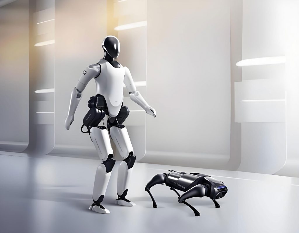
The operational principle of this bionic robot hinges on sophisticated motion analysis and biological inspiration. I applied kinematics analysis methods to enhance the stability margin during the maximum stride of a wave gait. This ensures that when the bionic robot walks at different speeds, the motor control parameters for the body can be corrected in real-time, guaranteeing stable locomotion. Furthermore, I employed a bionic research approach, utilizing the organizational coordination method of Central Pattern Generators (CPGs) and the decomposition function of the motor center. A bionic control system tailored for quadruped robots serves as the primary motion control device, enabling coordinated leg movements. The integration of these principles is fundamental to the autonomous function of the bionic robot.
The hardware architecture of the bionic robot is divided into mechanical and electrical subsystems, both crucial for its functionality.
| Subsystem | Components | Description and Function |
|---|---|---|
| Mechanical Part | 3D-Printed Parts | All structural components (body, head, neck, legs) were fabricated using 3D printing technology, allowing for complex geometries and rapid prototyping. |
| Assembly Method | Larger structures like the head and neck are connected via screws. Joints in the legs are designed for servo motor actuation. | |
| Module Integration | A voice module and an ultrasonic module are housed in the head (top and eye sockets, respectively). | |
| Overall Design | The bionic robot exhibits coordinated proportions and stable movement potential. | |
| Electrical Part | Main Control Board | A dedicated motherboard governs all actions. It receives and executes programmed commands via Bluetooth. |
| Communication Modules | Bluetooth and Wi-Fi modules, along with the primary controller (Arduino), are located on the robot’s back. | |
| Power System | The drive system uses a 12V AC power source. Sensors operate on 3.6V DC. | |
| Control Interface | Supports remote operation via a smartphone app, which offers a simple, clear interface for detailed motion adjustment and precise management. |
The software infrastructure is the brain of the bionic robot. The main control flowchart governs its operation. I implemented three primary control methods to enhance the interactivity of this bionic robot: computer control via dedicated software, voice control within a 5-meter range for direct command execution, and smartphone control through a custom mobile application. This multi-modal control scheme makes the bionic robot highly accessible and user-friendly.
| Control Method | Range/Interface | Primary Functions |
|---|---|---|
| Computer Control | Direct USB/Serial connection | Low-level programming, gait tuning, system diagnostics. |
| Voice Control | ~5 meters, microphone input | Triggering pre-programmed action sequences via spoken commands. |
| Smartphone Control | Remote via Bluetooth/Wi-Fi, GUI App | Real-time motion control (forward, back, turn, etc.), action selection, parameter fine-tuning. |
The realization of this advanced bionic robot relied on several key technologies. First, system modeling combined with 3D printing was essential. I created a detailed model of the quadruped bionic robot based on the bovine walking cycle using SolidWorks. The modeling specifically focused on the sagittal plane, capturing phases such as the front legs contacting and compressing while the rear legs are unloaded, and both front and rear legs being in contact. This model was then physically realized using 3D printing technology, which allowed for the rapid and cost-effective production of all custom parts. This synergy between digital modeling and additive manufacturing is a cornerstone of modern bionic robot development.
Second, Arduino control technology provided the flexible and accessible nervous system for the bionic robot. The Arduino platform, comprising both hardware (the Arduino Nano board) and software (the Arduino IDE), is an open-source electronic prototyping environment known for its ease of use. I employed it to develop the core control programs. This system allows for meticulous adjustment of the bionic robot’s movements, enabling precise management during operation and promoting the development of simpler and more refined control systems. The programmability of the Arduino is what赋予 this bionic robot its versatile behaviors.
A critical technical challenge involved the calculation of leg postures for stable gait generation. The bionic robot’s program primarily manages two key postures: the walking posture and the marching-in-place posture. Each requires distinct computational formulas. The foundation for these calculations is the servo calibration position, where the leg and foot form a straight line perpendicular to the ground and the body. The relevant geometric parameters are defined as follows:
- $H$: Vertical distance from the hip servo axis to the ground.
- $L_{\text{hip}}$: Distance from the hip servo axis to the ankle servo axis.
- $L_{\text{leg}}$: Distance from the ankle servo axis to the tip of the foot.
These lengths ($L_{\text{hip}}$ and $L_{\text{leg}}$) are constants measured from the physical parts, while $H$ is a setpoint for the desired standing height. For the marching-in-place posture, the leg must move such that the line from the hip servo axis to the foot tip remains vertical. This requires maintaining a constant effective leg length $L$ and ensuring it stays perpendicular to $H$. If we let $a$ be the real-time angle deviation of the hip servo from its calibration position (in radians), and $(b + a)$ be the corresponding deviation for the ankle servo, their relationship can be derived from geometry.
The core kinematic relationship for the leg in the sagittal plane, ensuring the foot tip remains directly below the hip during a vertical lift phase, can be expressed. The effective length $L$ is the hypotenuse when the leg is not vertical. However, for the specific marching case described (keeping the leg line vertical), the condition is simpler. The angles $a$ and $b$ must compensate for each other to keep the foot directly under the hip projection. A more general formula for calculating servo angles to achieve a desired foot position $(x, z)$ relative to the hip joint in a 2D model is:
For a two-segment leg (thigh of length $L_t$ and calf of length $L_c$), the inverse kinematics can be solved. Let the hip joint be at (0,0), the knee at $(x_k, z_k)$, and the foot at $(x_f, z_f)$. We can define $L_t = L_{\text{hip}}$ and $L_c = L_{\text{leg}}$. The distance from hip to foot is $D = \sqrt{x_f^2 + z_f^2}$. The angle of the hip joint relative to vertical, $a$, and the internal knee angle are calculated using the law of cosines:
$$ \theta_{\text{knee}} = \arccos\left(\frac{L_t^2 + L_c^2 – D^2}{2 \cdot L_t \cdot L_c}\right) $$
$$ a = \arctan2(x_f, z_f) \mp \arccos\left(\frac{L_t^2 + D^2 – L_c^2}{2 \cdot L_t \cdot D}\right) $$
The sign depends on the leg configuration (elbow-up or elbow-down). In our calibrated zero position, $a=0$, $b=0$, $x_f=0$, and $z_f = -(L_{\text{hip}} + L_{\text{leg}}) = -H_{\text{max}}$. During marching, if we want the foot to move vertically while the hip stays fixed, then $x_f=0$ and $z_f = -H_{\text{set}}$. The formulas simplify. For the bionic robot’s specific case, the relationship between $a$ and $b$ to maintain a straight, vertical leg ($x_f=0$) is complementary: $b = -a$. This ensures the foot segment rotates opposite to the thigh to keep the overall leg line straight. The actual commanded servo angles, $\alpha_{\text{cmd}}$ and $\beta_{\text{cmd}}$, are then:
$$ \alpha_{\text{cmd}} = \alpha_{\text{cal}} + a $$
$$ \beta_{\text{cmd}} = \beta_{\text{cal}} + b = \beta_{\text{cal}} – a $$
where $\alpha_{\text{cal}}$ and $\beta_{\text{cal}}$ are the servo pulse-width values corresponding to the calibrated zero angles. A critical implementation detail involves unit conversion and calibration. In Arduino programming, trigonometric functions require angles in radians. The conversion is:
$$ \text{radians} = \text{degrees} \times \frac{\pi}{180} $$
Furthermore, for the 9g servo motors used, a linear scaling error was identified and compensated for:
$$ \text{Actual Angle (degrees)} \approx 0.9 \times \text{Input Command Value} $$
This relationship is servo-dependent. Due to measurement errors and servo nonlinearities, empirical compensation constants $C_{\text{hip}}$ and $C_{\text{ankle}}$ were added to the calculated angles in the final code to achieve smooth and balanced motion for the bionic robot:
$$ \alpha_{\text{final}} = \alpha_{\text{cmd}} + C_{\text{hip}} $$
$$ \beta_{\text{final}} = \beta_{\text{cmd}} + C_{\text{ankle}} $$
These constants were determined through iterative testing on the physical bionic robot, not derived analytically. This pragmatic approach is common in refining the performance of a complex bionic robot.
| Symbol | Description | Unit |
|---|---|---|
| $H$ | Desired height from hip axis to ground | mm |
| $L_{\text{hip}}$ | Length of thigh (hip to ankle joint) | mm |
| $L_{\text{leg}}$ | Length of foot segment (ankle to foot tip) | mm |
| $a$ | Hip servo angle offset from calibration (radians) | rad |
| $b$ | Ankle servo angle offset from calibration (radians) | rad |
| $C_{\text{hip}}, C_{\text{ankle}}$ | Empirical compensation constants | Unitless (scaled to command units) |
| $\alpha_{\text{cmd}}, \beta_{\text{cmd}}$ | Calculated servo command values | PWM units |
The technical performance specifications of the developed bionic robot are comprehensive. The range of actions it can perform includes, but is not limited to: sitting, shaking hands (via a leg gesture), following an object (using the ultrasonic sensor), marching in place, standing, walking forward, walking backward, turning left, turning right, stopping, performing a swaying motion, lying down and standing up, autonomous walking, and even kicking a ball. This diverse action repertoire demonstrates the versatility of this bionic robot platform.
| Category | Indicator | Details |
|---|---|---|
| Motion | Locomotion Gaits | Static walk, in-place march. |
| Discrete Actions | Sit, stand, lie down, shake, sway, kick. | |
| Maneuverability | Forward, backward, left/right turn on the spot. | |
| Hardware | Drive Power | 12V AC source for servo motors. |
| Sensor Power | 3.6V DC for ultrasonic and voice modules. | |
| Core Controller | Arduino Nano microcontroller board. | |
| Interaction | Control Range | Voice: ~5m; Bluetooth/Wi-Fi: dependent on environment. |
In conclusion, the development of this bionic robot has been a profoundly educational and successful endeavor. Compared to many commercial robots available on the market, this bionic robot exhibits a significant advantage in cost due to the use of system modeling combined with 3D printing technology, which drastically reduces material and prototyping expenses. Regarding stability and performance, the capabilities of this bionic robot are comparable to existing market offerings, successfully achieving stable walking and a variety of interactive behaviors. The integration of bionic principles, accessible control technology, and additive manufacturing makes this bionic robot an excellent platform for STEM education, capable of stimulating student interest in robotics and engineering through simple operation. The potential applications for such a bionic robot extend beyond education into areas like entertainment, basic research in locomotion, and as a testbed for sensor integration. Future work on this bionic robot could involve integrating more advanced sensors (e.g., IMUs for dynamic balance), implementing more adaptive CPG-based algorithms, and exploring dynamic gaits like trotting. The journey of designing and building this bionic robot reaffirms the immense value of bionic inspiration in pushing the boundaries of robotic systems.