
In the evolution of robotics, wheeled and tracked robots first broke through the limitations of traditional design and opened the exploration of robotic technologies. With the continuous development of bionics, legged robots have gradually evolved toward simulating biological movement mechanisms. Bipedal and quadrupedal robots imitate the locomotion of birds and mammals respectively, demonstrating significant advantages in moving over uneven terrain and carrying loads efficiently. Currently, robots are increasingly moving toward higher anthropomorphism. Under the strategic background of “Made in China 2025” and “Industry 4.0”, highly anthropomorphic humanoid robots show greater flexibility and adaptability in tasks such as collaboration, assembly, and maintenance. How to provide sufficient human motion data suitable for a humanoid robot has become a critical issue in anthropomorphic motion control and action learning. However, human topology and mass distribution differ from those of a humanoid robot, so human motion data cannot be directly used to drive and make a humanoid robot learn actions. These problems seriously limit the realization of anthropomorphic behaviors.
To solve the above problems, this dissertation first proposes a human motion data segmentation and synthesis technique to achieve the reuse of limited data and construct a set of human motion data suitable for a humanoid robot to imitate. Then, an action mapping and retargeting method based on human motion data is proposed to address the accuracy and fluency problems in action generation of existing techniques. The main contents are as follows:
1. A kinematic model of the Qinglong humanoid robot is established. Based on the D-H method, coordinate transformation relationships between different coordinate systems are established, and the mapping relationship between the limb workspace and joint space is deduced and verified. The limb workspace is analyzed to clarify the anthropomorphic action range of the Qinglong humanoid robot.
2. A human motion data segmentation method based on spatio-temporal characteristics is proposed. First, human motion data in multiple behavioral scenarios are collected by an inertial motion capture suit, and combined with multi-behavior data selected from the Carnegie Mellon University (CMU) motion capture database. Time-series features and spatial trajectory changes are extracted to realize accurate segmentation of complex multi-behavior data. To further enrich human motion data applicable to a humanoid robot, the segmented motion clips are constructed as an arbitrarily spliceable motion graph to enhance the flexibility and extensibility of action data. In addition, a quaternion interpolation method is used to optimize the motion data to ensure natural and smooth transition effects.
3. To realize the action design of the Qinglong humanoid robot and the mapping and retargeting from human behavior to robot actions, the Blender platform is used to build a high-precision three-dimensional animation model of the Qinglong humanoid robot. A robot action design method based on keyframe interpolation and skeleton binding is proposed. Specifically, cubic Bezier curve interpolation and cyclic gradient descent are used to achieve precise planning of robot action trajectories. Meanwhile, to solve the retargeting problem from human motion data to robot actions, an action mapping method based on segmented kinematics and quadratic programming is proposed. This method combines a segmented kinematic model and quadratic programming to optimally adjust the robot action trajectory, thereby achieving effective mapping between human motion features and robot motion constraints. Subsequently, the proposed method is visually verified on the Blender platform. Experimental results show that the method can effectively complete the action retargeting task and generate robot motion trajectories that meet expectations. To further verify the applicability and realism of the motion data, the motion data after quadratic programming are applied to the robot control system in the Webots simulation environment. Experimental results show that the humanoid robot in the Webots simulation environment can accurately execute actions according to the planned trajectory, while exhibiting high motion stability and environmental adaptability.
1 Introduction
Robot technology is a high-tech field that integrates mechanical engineering, electronic technology, computer science, and artificial intelligence. It is one of the important technologies driving social productivity transformation. Humanoid robots, as an important branch of robotics, have gradually become a research hotspot. A humanoid robot usually has bipedal legs, dual arms, and a human-like joint distribution. It can imitate the human body shape and realize functions such as standing, walking, grasping, and manipulation. Compared with quadruped robots, a humanoid robot has higher degrees of freedom and flexible motion ability. Therefore, humanoid robots have broad application prospects in service robotics, medical rehabilitation, education and entertainment, disaster rescue, and other fields.
At present, although humanoid robots show certain motion abilities, they still cannot be directly applied to real environments and cannot perfectly reproduce human motion. One reason is that the trajectories of humanoid robots do not fully refer to real human motion data. Usually, there are two methods for trajectory generation of humanoid robots: one is trajectory planning based on high-precision mathematical models (dynamic modeling, kinematic modeling), which requires constructing complex constraint conditions and solving nonlinear optimization problems. The computational complexity increases exponentially with the number of robot degrees of freedom. The other is teaching by demonstration, in which an operator manually drags the robot to move, records key path points, and then generates a continuous trajectory through interpolation algorithms. This process is costly. In this context, exploring human action mapping and retargeting technology that combines the advantages of teaching learning and trajectory optimization has important research value for improving industrial task adaptability in complex scenarios.
Action teaching is a reliable form for non-expert users to control a humanoid robot, and motion segmentation and understanding of human action data are its prerequisites. When using existing methods to perform keyframe extraction and motion segmentation on captured raw human motion data, due to unclear data characteristics, it is difficult to accurately locate the start frame, end frame, and segmentation frame. This affects the robot’s learning from teaching data and makes it impossible to achieve control purposes. In this case, studying segmentation algorithms and motion clip combination technology is of great practical significance. At the motion control level, the movement of a humanoid robot requires the coordination of the torso, legs, and robotic arms to achieve whole-body cooperative motion in complex dynamic environments. This process inevitably faces the following challenges: multi-degree-of-freedom dynamic balance, environmental interaction adaptability, and energy efficiency optimization. To address these challenges, it is of great research significance to realize motion control of a humanoid robot and make full use of its redundant degrees of freedom while ensuring trajectory tracking accuracy.
2 Humanoid Robot System and Modeling
2.1 System Description
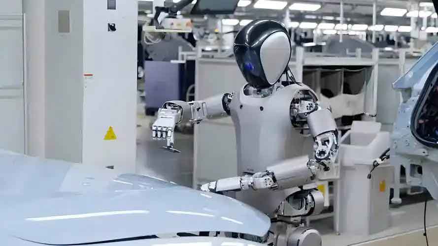
This research adopts the Qinglong full-size general-purpose humanoid robot as the research object. The Qinglong humanoid robot is a high-performance humanoid robot independently developed in China. Its design has a highly bionic torso structure. The whole machine can have up to 43 degrees of freedom, and the maximum joint peak torque reaches 396 N·m. The overall height of the robot is about 1.85 m and its weight is about 80 kg. It exhibits diverse motion abilities, including fast walking, flexible obstacle avoidance, robust slope climbing, and anti-impact disturbance. These characteristics make it an ideal carrier for general artificial intelligence applications.
According to the Chinese national standard GB10000-88, for males aged 18 to 25 in East China with a height of 180 to 185 cm, the thigh length is about 532 mm, the shank length is about 421 mm, the upper arm length is about 350 mm, and the forearm length is about 269 mm. The robot structure design refers to these data.
The degrees of freedom configuration of the whole robot is shown in Table 1. The head has 2 degrees of freedom, including 2 neck joints. Each leg has 6 degrees of freedom, including 3 hip joints, 1 knee joint, and 2 ankle joints. Each arm has 7 degrees of freedom, including 3 shoulder joints, 1 elbow joint, and 3 wrist joints. The two dexterous hands each have 6 degrees of freedom.
| Joint group | Degrees of freedom |
|---|---|
| Head | 2 |
| Leg | 6 × 2 |
| Waist | 3 |
| Arm | 7 × 2 |
| Dexterous hand | 6 × 2 |
2.2 Spatial Transformation Description
When describing the state of a robot in space, position and orientation are usually expressed by two variables. By establishing coordinate systems on each robot component and describing the transformation between coordinate systems, the motion relationship of robot components is expressed. Therefore, a position vector and a rotation matrix can describe the motion of the robot.
Given a point $P$ expressed in coordinate system $\{C\}$ as ${}^{C}P$, its expression in coordinate system $\{A\}$ can be derived by chained transformations:
$$ {}^{C}P = {}^{C}_{B}T \, {}^{B}P $$
$$ {}^{B}P = {}^{B}_{A}T \, {}^{A}P $$
$$ {}^{A}P = {}^{A}_{B}T \, {}^{B}_{C}T \, {}^{C}P $$
Thus, the transformation matrix from $\{C\}$ to $\{A\}$ is:
$$ {}^{A}_{C}T = {}^{A}_{B}T \, {}^{B}_{C}T $$
In matrix form,
$$ {}^{A}_{C}T = \begin{bmatrix} {}^{A}_{B}R \, {}^{B}_{C}R & {}^{A}_{B}R \, {}^{B}P_{C\,org} + {}^{A}P_{B\,org} \\ 0_{1\times 3} & 1 \end{bmatrix} $$
The basic rotations about the X, Y, and Z axes are:
$$ R_x(\alpha) = \begin{bmatrix} 1 & 0 & 0 \\ 0 & \cos\alpha & -\sin\alpha \\ 0 & \sin\alpha & \cos\alpha \end{bmatrix} $$
$$ R_y(\beta) = \begin{bmatrix} \cos\beta & 0 & \sin\beta \\ 0 & 1 & 0 \\ -\sin\beta & 0 & \cos\beta \end{bmatrix} $$
$$ R_z(\gamma) = \begin{bmatrix} \cos\gamma & -\sin\gamma & 0 \\ \sin\gamma & \cos\gamma & 0 \\ 0 & 0 & 1 \end{bmatrix} $$
Quaternions are also used to represent orientation. A quaternion is defined as:
$$ q = w + xi + yj + zk $$
with the constraint $w^2+x^2+y^2+z^2=1$. The rotation matrix corresponding to a quaternion rotating an angle $\theta$ about an arbitrary axis is:
$$ R(q) = \begin{bmatrix} 1-2(y^2+z^2) & 2(xy-wz) & 2(xz+wy) \\ 2(xy+wz) & 1-2(x^2+z^2) & 2(yz-wx) \\ 2(xz-wy) & 2(yz+wx) & 1-2(x^2+y^2) \end{bmatrix} $$
2.3 D-H Coordinate System Establishment
The Denavit-Hartenberg (D-H) method is a standard approach for robot kinematic modeling. In this method, four parameters $a_i$, $\alpha_i$, $d_i$, and $\theta_i$ are defined for each link. The transformation from frame $i-1$ to frame $i$ is given by:
$$ {}^{i-1}_{i}T = \begin{bmatrix} \cos\theta_i & -\sin\theta_i \cos\alpha_i & \sin\theta_i \sin\alpha_i & a_i \cos\theta_i \\ \sin\theta_i & \cos\theta_i \cos\alpha_i & -\cos\theta_i \sin\alpha_i & a_i \sin\theta_i \\ 0 & \sin\alpha_i & \cos\alpha_i & d_i \\ 0 & 0 & 0 & 1 \end{bmatrix} $$
For the Qinglong humanoid robot, four D-H tables are provided in the appendix of the original dissertation: left upper limb, right upper limb, left lower limb, and right lower limb. Each limb is modeled as a chain of links and joints. For example, the left arm has 7 degrees of freedom and the left leg has 6 degrees of freedom. The D-H parameters are too lengthy to list completely here, but the transformation matrices are used to derive forward kinematics.
2.4 Forward Kinematics Derivation
The forward kinematics of the left arm can be obtained by multiplying the individual transformation matrices:
$$ {}^{0}_{19}T = {}^{0}_{1}T \, {}^{1}_{2}T \, {}^{2}_{3}T \, {}^{3}_{4}T \, {}^{4}_{5}T \, {}^{5}_{6}T \cdots {}^{18}_{19}T $$
The position of the left arm end effector in the base frame is a function of six joint angles:
$$ \begin{bmatrix} p_x \\ p_y \\ p_z \end{bmatrix} = \begin{bmatrix} f_1(\theta_1,\theta_2,\theta_3,\theta_4,\theta_5,\theta_6) \\ f_2(\theta_1,\theta_2,\theta_3,\theta_4,\theta_5,\theta_6) \\ f_3(\theta_1,\theta_2,\theta_3,\theta_4,\theta_5,\theta_6) \end{bmatrix} $$
These functions are highly nonlinear expressions involving products of sines and cosines of the joint angles. They are listed in the appendix of the original thesis.
2.5 Forward Kinematics Verification
To verify the correctness of the forward kinematics model, I compared the end effector positions computed by the theoretical formulas with those extracted from the Blender model. The Blender model was driven by the same joint angles, and the resulting end effector positions were extracted. The comparison showed errors at the centimeter level. The small discrepancies are mainly caused by geometric parameter errors and numerical computation precision. For the lower limb, a constant error of 0.03 m in the Y direction was observed. After further investigation, I found that the error originated from the selection of the outermost point during parameterization. Because the error was constant, it could be compensated by an offset correction. Overall, the forward kinematics model is sufficiently accurate for motion retargeting.
2.6 Jacobian Matrix
The Jacobian matrix maps joint velocities to end effector velocities:
$$ \dot{X} = J \dot{q} $$
where $\dot{X}$ is the generalized velocity of the end effector, $J$ is the Jacobian matrix, and $\dot{q}$ is the joint velocity vector. For the left arm, the Jacobian is a $6 \times 6$ matrix whose entries are partial derivatives of the position components with respect to the joint angles:
$$ J = \begin{bmatrix} \frac{\partial p_x}{\partial \theta_1} & \frac{\partial p_x}{\partial \theta_2} & \cdots & \frac{\partial p_x}{\partial \theta_6} \\ \frac{\partial p_y}{\partial \theta_1} & \frac{\partial p_y}{\partial \theta_2} & \cdots & \frac{\partial p_y}{\partial \theta_6} \\ \frac{\partial p_z}{\partial \theta_1} & \frac{\partial p_z}{\partial \theta_2} & \cdots & \frac{\partial p_z}{\partial \theta_6} \\ \frac{\partial \phi_x}{\partial \theta_1} & \frac{\partial \phi_x}{\partial \theta_2} & \cdots & \frac{\partial \phi_x}{\partial \theta_6} \\ \frac{\partial \phi_y}{\partial \theta_1} & \frac{\partial \phi_y}{\partial \theta_2} & \cdots & \frac{\partial \phi_y}{\partial \theta_6} \\ \frac{\partial \phi_z}{\partial \theta_1} & \frac{\partial \phi_z}{\partial \theta_2} & \cdots & \frac{\partial \phi_z}{\partial \theta_6} \end{bmatrix} $$
This Jacobian is used in the quadratic programming based retargeting method described in Chapter 5.
2.7 Workspace Analysis
The workspace of a robot is the set of all positions reachable by the end effector. For the Qinglong humanoid robot, the workspace can be computed by using the forward kinematics formulas with a recursive assignment method. In this study, I used a step angle of 15 degrees to reduce computational complexity. The resulting workspace of the upper limbs is approximately spherical, allowing the arms to perform a wide variety of human-like motions. The workspace of the lower limbs is approximately hemispherical, with some unreachable regions. This means that the humanoid robot can reproduce most human lower limb motions, though some extreme poses may be difficult to realize.
3 Human Motion Data Segmentation and Synthesis Based on Spatio-Temporal Feature Extraction
3.1 Motion Data Acquisition
I acquired human motion data from two sources. The first source is the Xsens MVN Analyze inertial motion capture system. The device is equipped with 17 high-precision inertial sensors attached to the head, waist, and key parts of the limbs. During the test, a series of movements was captured, including squatting, kicking, jumping in place, slow walking, and running. The total number of frames is 6274, containing 8 types of actions. The second source is the CMU motion capture database, which includes a wide range of movements such as daily actions, sports actions, performing arts, and special performances. The CMU dataset is particularly useful for motion synthesis because many clips contain single actions.
3.2 Data Preprocessing
The raw motion data are stored in BVH files. The BVH file contains a HIERARCHY section describing the skeleton structure and a MOTION section containing the motion data. Each frame contains the global position of the root and the rotation channels of each joint. The rotation order is typically ZXY. To compute foot positions in the world coordinate system, I used the hierarchy transformation:
$$ {}^{O}_{F}T = {}^{O}_{R}T \, {}^{R}_{B}T \, {}^{B}_{T}T \, {}^{T}_{S}T \, {}^{S}_{F}T $$
where $R$, $B$, $T$, $S$, $F$ denote root, buttock, thigh, shin, and foot, respectively. The position of the ankle in the world frame is then:
$$ {}^{O}P_F = {}^{O}_{B}R \, {}^{B}_{T}R \, {}^{T}_{S}R \, \text{offset}_F + {}^{O}_{T}R \, {}^{T}_{S}R \, \text{offset}_S + {}^{O}_{S}R \, \text{offset}_T + {}^{O}_{B}R \, \text{offset}_B + {}^{O}P_R $$
The center of mass (COM) is calculated by averaging the segment centers weighted by their masses:
$$ P_{com} = \frac{\sum_i m_i P_i}{\sum_i m_i} $$
where $m_i$ are the relative masses of body segments according to Table 2.
| Segment | Relative mass (%) |
|---|---|
| Head and neck | 8.62 |
| Upper torso | 16.82 |
| Lower torso | 27.23 |
| Thigh | 14.19 |
| Shank | 3.67 |
| Upper arm | 22.43 |
| Forearm | 1.25 |
| Hand / foot | 0.64 / 1.48 |
3.3 Spatio-Temporal Feature Extraction
3.3.1 Dynamic Balance Features
The dynamic balance features are extracted using a simplified inverted pendulum model. The pendulum length $r$ is the distance from the COM to the support foot:
$$ r = \sqrt{(x_{com} – x_f)^2 + (z_{com} – z_f)^2} $$
The pendulum angle $\theta$ is the angle of the COM relative to the vertical direction in the sagittal plane:
$$ \theta = \arctan\left(\frac{z_{com} – z_f}{x_{com} – x_f}\right) $$
The COM velocity and acceleration are obtained by numerical differentiation:
$$ V_{com} = \dot{P}_{com}, \quad A_{com} = \ddot{P}_{com} $$
These features provide dynamic information that helps distinguish different motion phases.
3.3.2 Gait Periodicity Features
Gait features include foot support state, step length, stride length, step height, gait cycle, and duty cycle. The support state is determined by thresholding the vertical positions of the left and right ankles. Four states are defined: double support (0), left support (1), right support (2), and no support (3).
The step length $h$ is the distance in the X direction between the left and right feet:
$$ h = |x_{rf} – x_{lf}| $$
The stride length is calculated as the distance traveled from one support phase to the next support phase of the same foot:
$$ s = z_{n+1}^{lf} – z_n^{lf} $$
The step height is the maximum height of the foot during a gait cycle:
$$ d_h = \max |y_{foot_i} – y_{ground}| $$
The duty cycle is the ratio of the summed support time to the gait cycle duration:
$$ D = \frac{\sum_{j} D_{Rj}}{\text{frames per cycle}} $$
where $D_{Rj} = \frac{s_j}{2}$ and $s_j$ is the number of supporting feet at frame $j$.
3.4 Motion Data Construction and Segmentation
After extracting spatio-temporal features, each frame is represented by a 69-dimensional vector:
$$ \mathbf{f}_i = \begin{bmatrix} P_{com} & V_{com} & A_{com} & \theta & r & D & h & h_s & d_h & o_1 & \cdots & o_{18} \end{bmatrix}^T $$
where $o_1, \dots, o_{18}$ are the original joint rotations of the 18 joints. The full data matrix is:
$$ F = \begin{bmatrix} \mathbf{f}_1 & \mathbf{f}_2 & \cdots & \mathbf{f}_m \end{bmatrix}^T $$
To segment the motion sequence, I used probabilistic principal component analysis (PPCA). First, the data are centered:
$$ \mathbf{f}’_i = \mathbf{f}_i – \bar{\mathbf{f}} $$
where $\bar{\mathbf{f}} = \frac{1}{m} \sum_{i=1}^m \mathbf{f}_i$. Then singular value decomposition is performed on the centered matrix $Y$:
$$ Y = U S V^T $$
The projection dimension $s$ is chosen by setting a threshold $\xi$:
$$ \xi_s = \frac{\sum_{j=1}^s \sigma_j^2}{\sum_{j=1}^{69} \sigma_j^2} > \tau $$
The noise variance is estimated by:
$$ \sigma^2 = \frac{1}{69-s} \sum_{i=s+1}^{69} \sigma_i^2 $$
The covariance matrix is:
$$ C = \frac{1}{m-1} (W W^T + \sigma^2 I) $$
where $W = V_s S_s – \sigma^2 I$.
The average Mahalanobis distance from frame $k$ to frame $k+T$ with respect to the first $k$ frames is:
$$ H = \frac{1}{T} \sum_{i=k}^{k+T} (\mathbf{f}_i – \bar{\mathbf{f}})^T C^{-1} (\mathbf{f}_i – \bar{\mathbf{f}}) $$
By sliding $k$ forward, a sequence of Mahalanobis distances is obtained. The peaks of this sequence correspond to motion transition points, i.e., segmentation frames. In my experiments, I set $\tau = 0.9$, $T = 300$, $k = T$, and the segmentation threshold $R = 60000$. The comparison of segmentation results under different parameters is shown in Table 3.
| R | τ | T | l | Precision P | Recall R |
|---|---|---|---|---|---|
| 10000 | 0.9 | 300 | 10 | 52.38% | 100% |
| 60000 | 0.9 | 300 | 10 | 88.8% | 100% |
| 80000 | 0.9 | 300 | 10 | 76.92% | 83.3% |
| 60000 | 0.8 | 300 | 10 | 71.43% | 83.3% |
Compared with a method that directly uses raw quaternion data and Mahalanobis distance, the proposed method improves both precision and recall. The comparison is shown in Table 4.
| Method | Correct split points A | Total split points Q | Manual split points M | Precision P | Recall R |
|---|---|---|---|---|---|
| Method in literature [15] | 8 | 10 | 12 | 80% | 66.7% |
| Proposed method | 12 | 14 | 12 | 88.8% | 100% |
3.5 Motion Synthesis
To generate long multi-task motion sequences, I constructed a motion graph from the segmented motion clips. Each motion node $M_i$ contains a sequence of frames $[m(0), m(1), \dots, m(t)]$. The transition between two motion clips is achieved by finding the best similar frame using a weighted Euclidean distance:
$$ d(F_{1n}, F_{2j}) = \sqrt{\sum_{i=1}^k w_i (\theta_{1ni} – \theta_{2ji})^2} $$
where $w_i$ are joint weights and $\theta$ are joint angles. The frame with the minimum distance is selected as the transition frame. To ensure a smooth transition, quaternion spherical linear interpolation (slerp) is used:
$$ \text{slerp}(q, p, t) = \frac{\sin((1-t)\theta)}{\sin\theta} q + \frac{\sin(t\theta)}{\sin\theta} p $$
where $\theta = \cos^{-1}(q \cdot p)$ and $t \in [0,1]$. For a sequence of quaternions, squad interpolation is used to obtain smooth paths:
$$ \text{squad}(q_i, q_{i+1}, s_i, s_{i+1}, t) = \text{slerp}(\text{slerp}(q_i, q_{i+1}, t), \text{slerp}(s_i, s_{i+1}, t), 2t(1-t)) $$
where $s_i$ is an auxiliary quaternion:
$$ s_i = q_i \exp\left( -\frac{\log(q_i^{-1} q_{i-1}) + \log(q_i^{-1} q_{i+1})}{4} \right) $$
3.6 Experimental Results
I tested the segmentation method on the collected motion sequence. The foot trajectories, COM velocity, COM acceleration, inverted pendulum length, and angle were analyzed. The results showed that different motion phases have distinct spatio-temporal characteristics. For example, during squatting and jumping, the inverted pendulum length changes significantly; during walking and running, the pendulum angle changes rapidly. The gait cycle detection produced 14 cycles, as shown in Table 5.
| Cycle | Frame range | Time (s) |
|---|---|---|
| 1 | 0-300 | 1.250 |
| 2 | 301-1400 | 4.580 |
| 3 | 1401-1950 | 2.290 |
| 4 | 1951-2400 | 1.871 |
| 5 | 2401-2735 | 1.392 |
| 6 | 2736-3222 | 2.025 |
| 7 | 3223-3739 | 2.150 |
| 8 | 3740-4127 | 1.623 |
| 9 | 4128-4500 | 1.550 |
| 10 | 4501-4800 | 1.246 |
| 11 | 4801-5510 | 2.954 |
| 12 | 5511-5895 | 1.600 |
| 13 | 5896-6136 | 1.000 |
| 14 | 6137-6274 | 0.571 |
Motion synthesis was verified by concatenating multiple motion clips, such as punching, cross-cutting, squatting with arm raising, arm swinging, and jumping. The joint angle curves of the shoulder, elbow, and knee were analyzed. The curves were smooth and continuous at the transition regions, with no steep or vertical fluctuations. This confirms that the quaternion interpolation method effectively prevents motion discontinuity and produces natural transitions.
4 Three-Dimensional Animation Model Construction and Setup
4.1 Platform Selection
To design and visualize motions of a humanoid robot, I selected Blender 4.0 as the three-dimensional animation platform. Blender is free, open-source, and supports Python scripting. It provides a complete 3D production pipeline including modeling, rigging, animation, simulation, and rendering. Compared with commercial software such as Maya, 3ds Max, and Cinema 4D, Blender’s open-source nature and Python API allow me to write custom plugins for trajectory extraction and robot control. A comparison of common 3D animation platforms is shown in Table 6.
| Platform | Modeling accuracy | Trajectory export | 3D production pipeline | Open source | Scripting language |
|---|---|---|---|---|---|
| Blender | High | Supported | Complete | Free and open source | Python |
| Maya | High | Supported | Complete | No | MEL, Python |
| 3ds Max | High | Supported | Complete | No | MaxScript |
| Cinema 4D | Medium | Supported | Complete | No | Python |
| Unity | Medium | Supported | Partial | Partial | C# |
| Unreal Engine | Medium | Supported | Complete | Partial | C++ |
4.2 Robot Model Construction
The Qinglong humanoid robot model was imported into Blender from its URDF file. To enhance compatibility, the URDF was converted to FBX format using a plugin. After import, the robot model consists of many mesh objects. However, these meshes are not connected as a rigid body tree. To create a functional animation model, I generated a bone for each moving part and set parent-child relationships according to the robot’s kinematic chain. The skeleton contains 30 bones in total: 6 bones for each leg, 7 bones for each arm, and 3 bones for the torso, plus additional bones for ends.
Each bone was constrained to rotate around its corresponding robot joint axis, and the rotation ranges were set according to the joint limits in Appendix Table 5 of the original dissertation. This ensures that the Blender model has exactly the same joint motion limitations as the real humanoid robot.
4.3 Coordinate System and Frame Rate Matching
To avoid inconsistencies between the Blender model and the simulated robot, I matched the coordinate systems. In Blender, the robot coordinate axes are denoted as $x_b$, $y_b$, $z_b$, where $x_b$ is the forward direction, $y_b$ is the left direction, and $z_b$ is the vertical direction. The robot coordinate system in the simulation environment is $x_v$, $y_v$, $z_v$. The transformation is:
$$ \begin{bmatrix} x_v \\ y_v \\ z_v \end{bmatrix} = \begin{bmatrix} 0 & 1 & 0 \\ -1 & 0 & 0 \\ 0 & 0 & 1 \end{bmatrix} \begin{bmatrix} x_b \\ y_b \\ z_b \end{bmatrix} $$
The frame rate in Blender was set equal to the controller frequency of the robot. If the frame rate is lower than the controller frequency, the robot will execute the trajectory faster than expected, causing instability. If it is higher, the robot will lag behind. Therefore, I set the Blender frame rate equal to the controller frequency to ensure accurate execution.
5 Humanoid Robot Behavior Design and Motion Retargeting
5.1 Keyframe-Based Behavior Design
I designed robot behaviors using keyframe interpolation and the function curve editor in Blender. The keyframe technique requires setting the robot’s pose at certain frames, and then Blender automatically interpolates the intermediate frames. To avoid the Runge phenomenon, I used cubic Bezier interpolation between keyframes. The cubic Bezier curve equation is:
$$ B(t) = (1-t)^3 P_0 + 3(1-t)^2 t P_1 + 3(1-t) t^2 P_2 + t^3 P_3 $$
where $t \in [0,1]$ is the normalized time, and $P_0, P_1, P_2, P_3$ are control points. By choosing appropriate control points, the motion trajectory remains smooth and accurate. For example, I designed an arm waving action by setting five keyframes at frames 1, 100, 200, 300, 400, and 500. The bones were rotated to the desired angles at each keyframe, and the interpolation generated a smooth motion.
5.2 Skeleton Binding Based Behavior Design
To retarget human motion data to the humanoid robot, I imported the synthesized human motion as BVH data into Blender. The human skeleton and the robot model were aligned, and IK constraints were applied to the robot’s limbs. Each leg had an IK chain with 6 bones, and each arm had an IK chain with 7 bones. The inverse kinematics solver used the cyclic coordinate descent (CCD) algorithm.
The CCD algorithm works as follows. Let $P_e$ be the current end effector position and $P_t$ the target position. The error vector is:
$$ \mathbf{e} = P_t – P_e $$
For each joint $k$, the adjustment angle is:
$$ \Delta\theta_k = \alpha \frac{\mathbf{e} \cdot \mathbf{v}_k}{\|\mathbf{v}_k\|^2} $$
where $\mathbf{v}_k$ is the direction vector of the joint’s rotation contribution, and $\alpha$ is a step constant. The algorithm iterates through all joints until the error norm is below a threshold:
$$ \|P_t – P_e\| < \epsilon $$
After IK solving, the robot can follow the human’s end effector trajectories. The robot’s torso follows the human root using child-of constraints.
5.3 Trajectory and Joint Angle Extraction
To extract the joint angles from the Blender animation, I used a method based on two auxiliary bones per joint: a test bone and a reference bone. The test bone follows the original bone, while the reference bone remains fixed at the initial pose. The joint angle is calculated from the angle between the two bone vectors:
$$ \theta_i = \arccos\left(\frac{\mathbf{t}_i \cdot \mathbf{b}_i}{\|\mathbf{t}_i\| \|\mathbf{b}_i\|}\right) $$
where $\mathbf{t}_i$ is the test bone vector and $\mathbf{b}_i$ is the reference bone vector. This method avoids the difficulty of directly reading IK-solved bone rotations from Blender API.
I also extracted trajectory information such as torso position, foot positions, and arm end effector positions for each frame. The exported trajectory information is summarized in Table 7.
| Trajectory category | Specific data type |
|---|---|
| Torso trajectory | COM position, COM velocity, torso orientation, torso angular velocity |
| Foot trajectory | Foot position, foot velocity, foot acceleration |
| Arm trajectory | Arm end pose, arm end velocity, arm end angular velocity |
5.4 Quadratic Programming Based Retargeting
To achieve automatic batch retargeting without manual editing, I proposed a method based on segmented kinematics and quadratic programming. I selected 14 key points on the human body and the humanoid robot, dividing the whole body into 9 kinematic chains. The mapping of positions is performed by scaling:
$$ P_r = \alpha P_h + \beta $$
where $\alpha = L_r / L_h$ is the ratio of robot limb length to human limb length, and $\beta$ is the offset. Orientation mapping uses a fixed rotation matrix:
$$ R_r = R^* R_h $$
The relative positions between adjacent key points are obtained. The relationship between the end effector velocity and joint velocity is:
$$ \dot{P} = J \dot{\theta} $$
To handle redundancy and joint limits, I formulated the retargeting as a quadratic programming problem:
$$ \min_{\dot{\theta}} \, (\mathbf{A}\dot{\theta} – \mathbf{b})^T Q (\mathbf{A}\dot{\theta} – \mathbf{b}) $$
subject to:
$$ \theta_{i\min} \leq \theta_i^{pre} + \dot{\theta}_i \Delta t \leq \theta_{i\max} $$
where $\mathbf{A}$ is the stacked Jacobian matrix, $\mathbf{b}$ is the desired end effector velocity, and $Q$ is a weighting matrix. The inequality constraints ensure that the joint angles remain within their mechanical limits.
I used the Gurobi optimizer to solve this QP problem at each time step. After obtaining the optimal joint velocities, I integrated them to update the joint angles:
$$ \theta(t+\Delta t) = \theta(t) + \dot{\theta}(t) \Delta t $$
Then the Jacobian is recomputed for the next step. The overall process is iterative and generates a full joint angle trajectory for the humanoid robot.
5.5 Experimental Validation in Blender
I validated the proposed methods in Blender. In the first 450 frames, the robot motion was generated by keyframe interpolation, and the remaining frames were generated by skeleton binding and IK solving. The results showed that the robot successfully performed a sequence of actions including upper limb motion, jumping, and forward motion. The root trajectory during the jumping motion exhibited a parabolic curve, which is physically reasonable. The upper limb end effector position of the robot closely followed the human upper limb trajectory. The lower limb end effector positions also matched well. The root trajectory is shown in Figure (not reproduced here) and indicated smooth transitions between actions.
5.6 Validation in Webots
To further verify the feasibility in a physical simulation environment, I applied the retargeted motion data to a Qinglong humanoid robot model in Webots. I implemented a proportional-derivative (PD) controller for joint motion tracking:
$$ \tau = K_p (\theta_d – \theta) + K_d (\dot{\theta}_d – \dot{\theta}) $$
where $K_p = 0.5$ and $K_d = 0.3$. The desired trajectories were obtained from the quadratic programming retargeting of the human action “palm strike – holding up the sky”. The simulation results showed that the robot successfully reproduced the human action in the Webots environment. Although the initial posture of the robot was sitting, which caused a vertical position offset in the arm trajectory, converting the global trajectory to the root-relative coordinate system revealed that the robot accurately followed the human motion. This demonstrates that the proposed retargeting method can handle the kinematic differences between the human and the humanoid robot and generate stable, natural motions.
6 Conclusion and Future Work
In this dissertation, I studied the motion retargeting problem for a humanoid robot based on human kinematic data. The main contributions are as follows:
(1) I established a kinematic model of the Qinglong humanoid robot using the D-H method. I derived and verified the forward kinematics and Jacobian matrix. The workspace analysis showed that the upper limbs have a spherical workspace, while the lower limbs have a hemispherical workspace with some unreachable regions. This clarifies the anthropomorphic movement range of the humanoid robot.
(2) I proposed a human motion data segmentation and synthesis method based on spatio-temporal feature extraction. By adding dynamic balance features and gait periodicity features to the raw motion data, the segmentation algorithm using probabilistic principal component analysis and Mahalanobis distance achieved higher precision and recall compared with existing methods. I also built a motion graph and used quaternion spherical interpolation to synthesize smooth multi-task motion sequences. This provides a richer and more diverse dataset for humanoid robot motion learning.
(3) I proposed two motion design and retargeting approaches for the Qinglong humanoid robot. The first relies on the Blender platform, using keyframe interpolation and skeleton binding with inverse kinematics. The second uses a quadratic programming formulation based on segmented kinematics. Both methods successfully map human motion data to the humanoid robot while respecting joint limits and maintaining smoothness. I validated the methods through animation in Blender and physical simulation in Webots. The results demonstrate that the humanoid robot can reproduce human actions with high fidelity and stability.
Future work will focus on the following aspects:
(1) The current methods are validated only in simulated environments. Future work should test them on the physical Qinglong humanoid robot, taking into account friction, collision, noise, and dynamic effects.
(2) The optimization algorithm is currently offline. To improve real-time performance, I plan to use deep learning based motion generation models and GPU acceleration.
(3) The human motion dataset should be expanded with more diverse and complex actions. A standardized and publicly available dataset would benefit the research community.
(4) The generated joint trajectories can be further refined using whole-body control methods such as model predictive control and whole-body control with dynamic constraints. Reinforcement learning can also be used to train policies that follow the reference trajectories while adapting to new environments.
In summary, this dissertation provides a systematic framework for human-like motion generation and retargeting of a humanoid robot, contributing to the development of advanced anthropomorphic robots in real-world applications.