
Humanoid robots have long been a symbol of advanced robotics, merging mechanics, electronics, control theory, computer vision, and artificial intelligence. In this thesis, I present a comprehensive study on the design of a humanoid robot controller and the development of gait control algorithms. The work covers hardware architecture, servo motor control, kinematic modeling, stability analysis, and practical gait generation. Throughout this research, the humanoid robot serves as the central platform for verifying theoretical results and experimental implementations.
1. Introduction and Research Background
The development of humanoid robots has progressed rapidly since the mid-20th century. Early industrial robots were designed for repetitive tasks such as welding, painting, and assembly. However, humanoid robots are fundamentally different: they are expected to operate in human-centered environments, using bipedal locomotion to navigate stairs, uneven terrain, and narrow spaces. The humanoid robot is a classic nonlinear, strongly coupled, and high-degree-of-freedom system. Therefore, the design of its controller and gait algorithm is both challenging and significant.
In this thesis, I focus on a small-scale humanoid robot with 20 degrees of freedom. The robot is designed to perform bipedal walking, track a colored ball, and provide voice feedback. To satisfy these requirements, a hierarchical control architecture is adopted. The main controller handles high-level tasks such as image processing and gait planning, while the motion controller executes low-level servo commands and sensor data acquisition.
The main contributions of this work are summarized as follows:
- Design of a complete humanoid robot controller including hardware and software.
- Selection and control design of digital servos for humanoid robot joints.
- Kinematic modeling using the Denavit-Hartenberg (D-H) method.
- Gait planning based on the Zero Moment Point (ZMP) criterion and the three-dimensional linear inverted pendulum model.
- Implementation of a practical action-frame-based gait generation method.
- Experimental validation on a physical humanoid robot prototype.
2. Humanoid Robot Controller Design
The controller of a humanoid robot must be able to process complex algorithms in real time while maintaining low power consumption and small physical size. In this design, I adopt a master-slave control architecture. The master controller is an industrial motherboard PICO-HC101, while the slave controller is based on an STM32 microcontroller. The communication between them is via USB-to-serial conversion. The overall software structure is divided into three layers: the main control module, the motion control module, and the execution module.
2.1 Main Controller Selection
The master controller needs to execute gait algorithms and image processing tasks. Therefore, I selected the PICO-HC101 industrial motherboard equipped with an Intel Atom processor. This board has a compact size of 56.5 mm × 66 mm, which is suitable for the limited space inside a humanoid robot. It provides multiple USB interfaces, serial ports, and supports a Linux operating system. The main features of the PICO-HC101 are listed in the following table:
| Feature | Description |
|---|---|
| Processor | Intel Atom E3845 / Celeron J1900 / N2807 |
| Display | Dual synchronous display, VGA up to 2048×1152, DP up to 2560×1400 |
| Storage | SATA 3.0 Gb/s, mSATA/Mini-Card |
| Serial Ports | COM1: RS-232, COM2: RS-232/422/485 |
| USB | USB 3.0 ×1, USB 2.0 ×2 |
| Audio | Line-out |
The choice of Linux as the operating system for the main controller is based on its open-source nature, low resource consumption, and support for real-time multitasking. I used Ubuntu 12.04 as the development platform, with C/C++ as the primary programming language.
2.2 Motion Control Board Hardware Design
The motion control board is the core of the lower-level control system. It is responsible for acquiring data from the gyroscope and accelerometer, controlling the servos, and maintaining real-time communication with the main controller. The board uses the STM32F103RET6 microcontroller, which has a 72 MHz ARM Cortex-M3 core, 256 KB flash memory, and 48 KB SRAM. The following table summarizes the STM32 specifications:
| Parameter | Value |
|---|---|
| Core | ARM 32-bit Cortex-M3 |
| Speed | 72 MHz |
| Program Memory | 256 KB Flash |
| RAM | 48 KB |
| Interfaces | CAN, I2C, SPI, UART, USB |
| Operating Voltage | 2.0 V – 3.6 V |
2.2.1 Crystal Oscillator and Reset Circuit
To ensure stable operation of the STM32, an 8 MHz quartz crystal oscillator is used as the external high-speed clock. The load capacitors are placed close to the oscillator pins to minimize noise. The reset circuit employs a simple RC network with a manual reset button, as the STM32 family has an internal pull-up resistor on the reset pin.
2.2.2 Power Supply Circuit
The humanoid robot is powered by an 11.1 V, 1800 mAh lithium battery. However, different modules require different voltage levels. The servo motors need 12 V, the communication circuits need 5 V, and the microcontroller and sensors need 3.3 V. Therefore, I designed two voltage regulation stages:
- From 11.1 V to 5 V: using the LM78M05 three-terminal regulator.
- From 5 V to 3.3 V: using the EZ1117 low-dropout regulator.
The power supply design must also handle the high current demand when all 20 servos operate simultaneously. The battery is selected to provide sufficient current without excessive weight.
2.2.3 Communication Circuit
The motion control board communicates with the main controller via USB. I selected the FT232 chip for USB-to-serial conversion because of its high reliability and compatibility. The communication between the motion control board and the servos uses TTL-level half-duplex asynchronous serial protocol. Additionally, I included an RS485 transceiver (MAX3440) for future expansion. The following table shows the serial communication parameters:
| Parameter | Value |
|---|---|
| Baud Rate | 1 Mbps (selected) |
| Data Bits | 8 |
| Stop Bits | 1 |
| Parity | None |
| Protocol | Half-duplex, packet-based |
2.2.4 Sensor Circuit
The stability of a humanoid robot relies on accurate orientation feedback. I used two sensors: a gyroscope (L3G4200D) and an accelerometer (LIS331DLH). These sensors interface with the STM32 via I2C or SPI. The gyroscope measures angular velocity, while the accelerometer measures linear acceleration. The combined data allows the controller to estimate the robot’s tilt angle. The measurement range of the gyroscope is ±500 dps, and the accelerometer range is ±4 g. The relationship between raw sensor values and physical units is linear, as shown in the following equations:
$$ \omega_{\text{dps}} = \frac{\text{raw\_gyro}}{16.4} $$
$$ a_{\text{g}} = \frac{\text{raw\_accel}}{4096} $$
These conversions are used in the firmware to obtain meaningful orientation data.
2.3 Actuator and Peripheral Design
The humanoid robot uses a Logitech C905 webcam for visual tracking. This camera has a 2-megapixel sensor and supports 1920×1080 resolution. It is connected to the main controller via USB. For audio output, I designed a speaker circuit based on the LM386 audio amplifier. The circuit provides voice prompts when the robot starts up or detects errors. Additionally, a microphone circuit using the LM324 operational amplifier is designed for future human-robot interaction.
2.4 PCB Design
After completing the schematic design, I created a four-layer PCB for the motion control board. The board layout places connectors on the edges for easy access, and the inertial sensors are located near the center to improve measurement accuracy. The PCB was fabricated and tested. The final board successfully provided power, communication, and sensor readout for the humanoid robot.
3. Servo Motor Control for the Humanoid Robot
The servo motor is the driving component of every joint in a humanoid robot. In this design, I selected the DYNAMIXEL MX-28T digital servo from ROBOTIS. This servo is compact but provides high torque and precise position control. It includes an STM32F103C8 microcontroller, a 12-bit absolute encoder, and supports a daisy-chain bus communication. The key specifications of the MX-28T are listed below:
| Parameter | Value |
|---|---|
| MCU | STM32F103C8, 72 MHz, 32-bit |
| Position Sensor | Contactless absolute encoder (12-bit, 360°) |
| Motor | Maxon Motor |
| Communication Speed | 8000 bps – 4.5 Mbps |
| Stall Torque (12V) | 2.5 N·m |
| No-load Speed (12V) | 55 r/min |
| Minimum Control Angle | 0.088° |
| Operating Voltage | 10 – 14.8 V |
3.1 Servo Communication Protocol
The MX-28T uses a half-duplex asynchronous serial protocol. The main controller sends an instruction packet to a specific servo ID, and the servo responds with a status packet. The packet format consists of the following fields:
| Bytes | Name | Description |
|---|---|---|
| 0xFF 0xFF | Header | Start of packet |
| ID | Servo ID | 0-253, broadcast allowed |
| LENGTH | Length | Number of parameters + 2 |
| INSTRUCTION | Instruction | Read, write, sync write, etc. |
| PARAMETERS | Parameters | Data for the instruction |
| CHECKSUM | Checksum | Complement of the sum of bytes |
To control multiple servos simultaneously, I used the SYNC WRITE instruction. This allows the master to send a single packet containing target positions for multiple servos, thereby minimizing communication delays. The synchronization of the humanoid robot’s joints is critical for coordinated walking.
3.2 Servo Control Table
The MX-28T has a control table stored in RAM and EEPROM, which defines the operational parameters. The most important RAM entries are:
| Address | Name | Description |
|---|---|---|
| 24 (0x18) | Torque ON/OFF | Enable/disable motor torque |
| 30 (0x1E) | Goal Position (L) | Target position low byte |
| 31 (0x1F) | Goal Position (H) | Target position high byte |
| 32 (0x20) | Moving Speed (L) | Target speed low byte |
| 36 (0x24) | Present Position (L) | Current position low byte |
| 42 (0x2A) | Present Voltage | Current voltage |
| 43 (0x2B) | Present Temperature | Current temperature |
The position value is a 12-bit integer in the range 0–4095, corresponding to 0°–360°. Thus the angular resolution is:
$$ \Delta \theta = \frac{360^\circ}{4096} \approx 0.0879^\circ $$
3.3 Servo ID Assignment
The humanoid robot has 20 servos positioned in the legs, arms, and torso. To simplify programming, I assigned servo IDs symmetrically. For example, the left and right shoulder pitch servos are assigned to ID 1 and ID 2, respectively. This symmetry allows code reuse and easier gait generation. The complete ID map is outlined in the following table:
| Joint | Left | Right |
|---|---|---|
| Shoulder pitch | 1 | 2 |
| Shoulder roll | 3 | 4 |
| Elbow pitch | 5 | 6 |
| Hip yaw | 7 | 8 |
| Hip roll | 9 | 10 |
| Hip pitch | 11 | 12 |
| Knee pitch | 13 | 14 |
| Ankle pitch | 15 | 16 |
| Ankle roll | 17 | 18 |
| Waist yaw | 19 | 20 |
3.4 Compliance Control for Smooth Motion
To reduce mechanical shock and improve walking smoothness, I implemented compliance parameters on each servo. The compliance margin and compliance slope affect torque near the target position. By adjusting these values, the humanoid robot can walk with less vibration. I experimentally determined the optimal compliance slope for one servo to be approximately 52, which minimizes the response time while maintaining accuracy.
4. Kinematic Modeling of the Humanoid Robot
Kinematics is the study of motion without considering forces. For a humanoid robot, forward kinematics computes the position and orientation of each link from joint angles, while inverse kinematics computes the joint angles required to achieve a desired pose. I used the D-H convention to establish coordinate frames for each joint.
4.1 Forward Kinematics
The humanoid robot can be modeled as a series of links connected by revolute joints. Starting from the supporting foot, coordinate frames are assigned to each joint according to the D-H parameters. The transformation from frame \(i\) to frame \(i-1\) is given by the homogeneous transformation matrix:
$$ T_i^{i-1} =
\begin{bmatrix}
\cos\theta_i & -\sin\theta_i \cos\alpha_i & \sin\theta_i \sin\alpha_i & a_i \cos\theta_i \\
\sin\theta_i & \cos\theta_i \cos\alpha_i & -\cos\theta_i \sin\alpha_i & a_i \sin\theta_i \\
0 & \sin\alpha_i & \cos\alpha_i & d_i \\
0 & 0 & 0 & 1
\end{bmatrix} $$
By multiplying the individual transformation matrices, the pose of the end-effector or any link can be obtained:
$$ T_n^0 = T_1^0 \, T_2^1 \, \cdots \, T_n^{n-1} $$
For a humanoid robot standing on the left foot, the right foot pose relative to the left foot is expressed by the product of transformations through the pelvis and both legs. This matrix is used to determine the foot placement during walking.
4.2 Inverse Kinematics
Inverse kinematics for a humanoid robot is more complex because multiple solutions may exist. I used a numerical iterative approach based on the Jacobian. The algorithm minimizes the error between the desired and current end-effector pose:
$$ \Delta p = p_{\text{ref}} – p_{\text{current}}, \quad \Delta R = R_{\text{ref}} R_{\text{current}}^T – I $$
The joint angle update is computed as:
$$ \Delta q = J^\dagger \begin{bmatrix} \Delta p \\ \Delta \phi \end{bmatrix} $$
where \(J^\dagger\) is the pseudo-inverse of the Jacobian matrix. Iteration continues until the pose error is below a threshold. This method is general and works well for the lower limb configuration of the humanoid robot.
5. Gait Planning and Control
Gait planning is the process of generating reference trajectories for the joints so that the humanoid robot walks stably. Two methods are investigated: the ZMP-based approach with a three-dimensional linear inverted pendulum model, and a practical action-frame method.
5.1 Zero Moment Point (ZMP)
The ZMP is defined as the point on the ground where the horizontal component of the moment due to gravity and inertial forces equals zero. If the ZMP remains inside the convex hull of the support polygon, the humanoid robot is dynamically stable. The ZMP coordinates can be computed from the robot’s mass distribution and accelerations:
$$ x_{\text{ZMP}} = \frac{\sum_{i} m_i ( \ddot{x}_i z_i – \ddot{z}_i x_i + g x_i ) – \sum_i I_{iy} \ddot{\Omega}_{iy}}{\sum_i m_i (\ddot{z}_i + g)} $$
$$ y_{\text{ZMP}} = \frac{\sum_{i} m_i ( \ddot{y}_i z_i – \ddot{z}_i y_i + g y_i ) – \sum_i I_{ix} \ddot{\Omega}_{ix}}{\sum_i m_i (\ddot{z}_i + g)} $$
In these equations, \(m_i\) is the mass of link \(i\), \((x_i,y_i,z_i)\) is its center of mass position, \(I_{ix}\) and \(I_{iy}\) are moments of inertia, and \(\Omega_{ix}, \Omega_{iy}\) are angular accelerations.
5.2 Three-Dimensional Linear Inverted Pendulum Model
A common simplification for humanoid robot walking is the three-dimensional linear inverted pendulum model. The robot is modeled as a point mass at the center of mass, supported by a massless leg. The contact point with the ground is considered frictionless, so there is no moment at the support point. The equation of motion in the horizontal plane is:
$$ \ddot{x} = \frac{g}{z_c} x, \quad \ddot{y} = \frac{g}{z_c} y $$
where \(z_c\) is the constant height of the center of mass. This linear differential equation has an analytical solution used for trajectory generation:
$$ x(t) = x_0 \cosh\left(\frac{t}{T_c}\right) + T_c \dot{x}_0 \sinh\left(\frac{t}{T_c}\right) $$
$$ \dot{x}(t) = \frac{x_0}{T_c} \sinh\left(\frac{t}{T_c}\right) + \dot{x}_0 \cosh\left(\frac{t}{T_c}\right) $$
where \(T_c = \sqrt{z_c / g}\). These equations allow the planner to compute the center of mass trajectory given boundary conditions. The following table shows representative walking parameters used in simulation:
| Parameter | Symbol | Value |
|---|---|---|
| Center of mass height | \(z_c\) | 0.45 m |
| Step length | \(S\) | 0.20 m |
| Step width | \(W\) | 0.15 m |
| Walking period | \(T\) | 1.0 s |
| Gravity acceleration | \(g\) | 9.81 m/s² |
Simulation results in MATLAB showed that the center of mass follows a smooth trajectory during both the double-support phase and the single-support phase. The ZMP remained inside the support polygon, confirming the stability of the planned gait.
5.3 Action-Frame-Based Gait Generation
Although the ZMP-based method is theoretically elegant, implementing it on the physical humanoid robot requires extensive computation and accurate dynamic models. As a practical alternative, I developed an action-frame-based method. In this approach, one walking cycle is decomposed into a sequence of key postures (frames). Each frame specifies the target angle for every servo. By playing these frames sequentially at a defined time interval, the humanoid robot moves through the walking cycle.
The walking cycle for one step includes the following frames:
- Initial upright standing.
- Bending knees to prepare for walking.
- Shifting center of mass to the left leg.
- Lifting the right foot.
- Moving the right foot forward.
- Lowering the right foot to the ground.
- Shifting the center of mass to the right leg.
- Repeating symmetrically for the left leg.
For each frame, the servo positions are computed using inverse kinematics or manually adjusted. The data is stored in a page on the main controller. A program allows the user to input each frame’s servo angles, set the playback time, and link pages. The gait generation process is implemented in Linux using a custom action editor.
Implementation Details
The action editor displays all current servo positions. The user can issue specific commands:
| Command | Function |
|---|---|
list |
List all action pages |
off [IDs] |
Set torque off for selected servos |
on [IDs] |
Set torque on for selected servos |
play |
Play the current action |
Time |
Set playback time for each frame |
Link to Next |
Connect to the next action page |
In my experiments, I created a walking cycle with 12 frames. The time for each frame was set to 125 ms, which gives a total cycle time of 1.5 seconds. After tuning the joint angles, the humanoid robot was able to walk forward stably. This method is intuitive and allows fast prototyping without complex dynamic modeling.
5.4 Comparison of Gait Planning Methods
I compared the ZMP-based three-dimensional inverted pendulum method and the action-frame method from various aspects. The following table summarizes the comparison:
| Criterion | ZMP + 3D-LIP | Action-Frame |
|---|---|---|
| Mathematical complexity | High | Low |
| Real-time computation | Requires fast solver | Simple lookup/playback |
| Adaptability | Can adapt to various terrains | Requires manual tuning |
| Stability guarantee | Stable if ZMP inside support | Empirical stability |
| Implementation effort | High | Moderate |
| Suitability for small robot | Simulation only | Successfully implemented |
The action-frame method was chosen for the physical humanoid robot due to its simplicity and the limited computational resources of the onboard controller. However, the ZMP-based method provides a solid theoretical foundation for future improvements, such as online gait adaptation and disturbance rejection.
6. Experimental Results
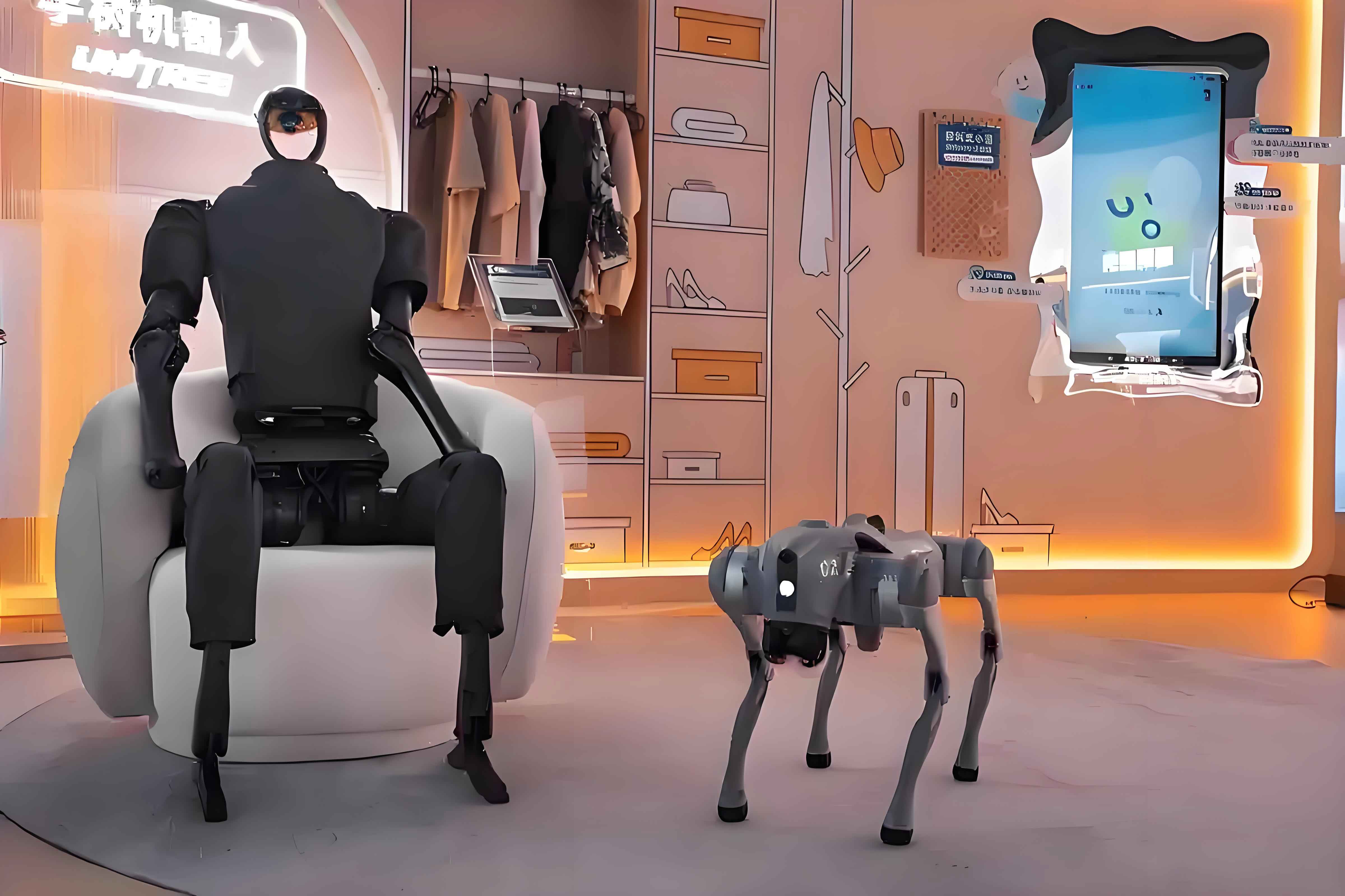
After completing the hardware assembly and software implementation, I tested the humanoid robot in various scenarios. The prototype stood about 50 cm tall and weighed approximately 2.5 kg. The robot was powered by a lightweight lithium battery. The following image shows a representative scene of the humanoid robot in a laboratory environment:
6.1 Walking Test
The action-frame-based gait was implemented and tested on the humanoid robot. The robot successfully performed a sequence of steps, maintaining balance and moving forward at a speed of about 0.13 m/s. The walking motion consisted of a preparatory squat, weight transfer, lifting and swinging the swinging leg, and landing. The arms were kept in a fixed posture to simplify the first test. The experiment demonstrated that the action-frame method is feasible for generating stable bipedal locomotion on a small humanoid robot.
6.2 Gyroscope and Accelerometer Calibration
To evaluate the sensor measurements, I collected data while the humanoid robot performed a forward fall. The gyroscope and accelerometer outputs were recorded and analyzed. The results showed that the gyroscope Y-axis data clearly indicated the forward rotation during the fall, while the accelerometer X-axis data showed the corresponding linear acceleration. The figures (omitted here) confirmed that the sensors function correctly and can provide reliable feedback for balance control.
The sensor readings can be used in a feedback controller to stabilize the humanoid robot. For example, when the robot tilts forward, the gyroscope detects angular velocity and the accelerometer detects gravity components. A simple proportional-derivative controller can adjust ankle torques to counteract the tilt.
7. Conclusion and Future Work
In this thesis, I presented a complete design and implementation of a humanoid robot controller, including hardware, software, servo control, kinematics, and gait planning. The main achievements are summarized as follows:
- Designed a master-slave controller architecture for a humanoid robot with 20 degrees of freedom.
- Implemented servo motor control using MX-28T digital servos with synchronized communication.
- Developed kinematic models using the D-H method and solved forward and inverse kinematics.
- Analyzed the ZMP stability criterion and simulated a 3D linear inverted pendulum based gait.
- Created a practical action-frame-based gait generator and demonstrated walking on the physical humanoid robot.
Future work will focus on improving the gait algorithm by integrating the ZMP-based method into the onboard controller, adding online balance feedback from the gyroscope and accelerometer, and optimizing the walking speed and smoothness. Additionally, vision-based ball tracking and voice interaction modules can be further developed to enhance the humanoid robot’s autonomy and human-robot interaction capabilities.
Overall, this research contributes to the field of humanoid robot control by providing a low-cost, flexible, and easily reproducible platform for gait experiments. The methods developed here can be extended to larger humanoid robots and more complex locomotion tasks.