
In the context of intelligent manufacturing transformation, industrial robots have become indispensable core execution equipment on automated production lines. The positioning accuracy of industrial robots is a core performance indicator that directly determines the execution quality and stability of tasks such as precision assembly, welding, and material handling. To address the insufficient characterization of the positioning accuracy error transfer mechanism of domestic industrial robots and the difficulty of implementing reliability evaluation under small-sample working conditions, I propose a positioning accuracy reliability analysis method for industrial robots based on meta-action decomposition. Taking a six-degree-of-freedom serial industrial robot as the research object, I first adopt the “Function–Movement–Meta-Action” decomposition method to decompose the whole machine into six single-degree-of-freedom meta-action units, and I use the Denavit–Hartenberg kinematic model to establish the static and dynamic displacement error models of each meta-action unit. Second, based on multi-body kinematics and the error Jacobian matrix, I construct an error transfer model from the meta-actions to the end effector. Then, I introduce the interval convex set model and the volume ratio method to complete the numerical calculation of positioning accuracy reliability. Finally, I carry out simulation verification through the MATLAB Robotics Toolbox. The results show that the forward kinematic model is accurate, the end-effector pose calculation is consistent with the simulation, the deviation between the error transfer model calculation and the simulation output is no more than 0.001 mm, and the deviation between the convex set model reliability and the Monte Carlo simulation result is no more than 3%. This method can clearly characterize the error transfer law and the reliability calculation of positioning accuracy, and it provides theoretical and methodological support for the accuracy design and reliability simulation of industrial robots.
The reliability of industrial robots is not merely a matter of control software or sensor feedback. It is rooted in the geometric and kinematic behavior of the mechanical structure itself. When industrial robots perform high-precision tasks, the accumulation of small displacement errors generated inside each joint eventually appears as an end-effector positioning error. Therefore, understanding how errors are generated at the lowest motion level and how they propagate along the kinematic chain is essential for improving the positioning accuracy reliability of industrial robots. My approach is to treat the complex machine as a collection of minimal motion units, which I call meta-actions, and to build a complete chain from unit decomposition to error modeling, error transfer, and reliability evaluation.
Current research on the positioning accuracy of industrial robots has covered three main directions: error transfer, error modeling, and reliability evaluation. The mainstream research methods are dominated by probabilistic statistics and fuzzy mathematics. However, research that combines whole-machine positioning accuracy reliability evaluation with low-level motion unit error analysis is still relatively scarce, and the framework of “unit decomposition–error modeling–transfer analysis–reliability analysis” has not been widely applied. A meta-action, as the smallest motion unit of a mechanical system, can achieve refined decomposition of complex mechanical systems and provides core theoretical support for low-level error analysis and reliability evaluation. In my work, I extend this idea to industrial robots and establish a systematic analysis route that connects the minimum motion unit to the end-effector accuracy.
1. Meta-Action Decomposition and Multi-Body System Description
To establish an expression model for the positioning accuracy of industrial robots from the perspective of error transfer, I need to decompose the complex whole-machine system into several motion units. I complete the decomposition of the industrial robot system based on the three-layer decomposition rule of “Function → Movement → Meta-Action,” and I establish the corresponding multi-body system model by combining the characteristics of the serial kinematic chain. This provides the structural basis for subsequent kinematic analysis and error analysis.
1.1 Meta-Action Theoretical Framework and Decomposition Logic
The core idea of meta-action theory is that “motion realizes function.” For the positioning accuracy reliability analysis of industrial robots, I adopt the meta-action decomposition rule to decompose the overall complex function of the robot into basic motion units that can be independently analyzed, level by level. The decomposition boundary is defined according to the transmission independence of the mechanical structure, so as to ensure that each meta-action unit is analyzable at the kinematic level. The decomposition follows the following criteria.
| Layer | Symbol | Description | Role in the analysis |
|---|---|---|---|
| Function layer | F | Describes the macro process task performed by the robot, such as assembly, welding, or spraying | Defines the overall functional boundary of the machine |
| Movement layer | M | Corresponds to the coordinated motion of each joint of the robot, completing complex spatial actions through the linkage of multiple components | Connects the macro function with the basic motion |
| Action layer | A | Constitutes the most basic, single-degree-of-freedom motion form of a component, namely the meta-action, driven by an independent power source | The smallest functional unit where displacement error is generated and transferred |
1.2 Meta-Action Decomposition of the Six-Axis Industrial Robot
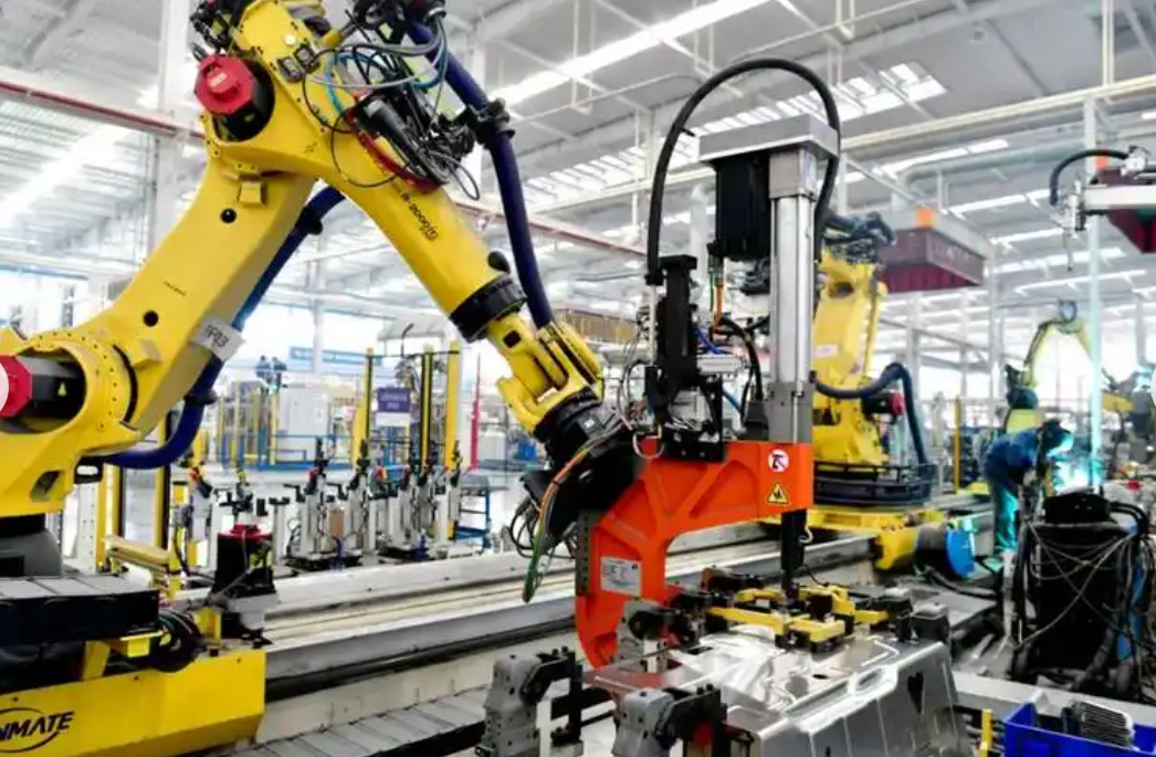
The six-axis serial industrial robot studied here is a typical serial machine. Its mechanical structure includes a base, a waist rotating body, an upper arm, a forearm, and a wrist with B, R, and T axes. The transmission system is composed of reducers, belts, gears, and other components. According to the meta-action decomposition logic, I complete the meta-action deconstruction of its positioning function. Because meta-action decomposition is only related to the structure of the industrial robot itself and the task function does not affect the decomposition process, I select a spraying task (F1) to divide the functional modules.
The motion control module (M) mainly performs precise positioning control of each joint in the space of six degrees of freedom. Its specific motion forms are waist rotation (M1), shoulder arm pitch (M2), forearm pitch (M3), wrist abduction and adduction (M4), wrist pronation and supination (M5), and wrist lateral swing (M6).
At the action layer (A), because the six-axis robot has six sets of independent drive joints, I obtain the following meta-actions: the waist body component rotation meta-action (A13), the upper arm body component swing meta-action (A23), the lower arm body component swing meta-action (A33), the wrist B-axis component rotation meta-action (A43), the wrist R-axis component swing meta-action (A53), and the wrist T-axis component rotation meta-action (A63). These six meta-actions correspond one-to-one to the active joints. They are all execution units in the meta-action chain and can directly change the end-effector pose. Therefore, six core meta-action units are obtained, and each unit realizes a single-degree-of-freedom motion, which serves as the basic unit for displacement error analysis.
| Index | Meta-action name | Input component | Output component | Supporting component | Fastening component | Intermediate component |
|---|---|---|---|---|---|---|
| A13 | Waist body rotation meta-action | No. 1 reducer flexspline | Waist body component | Base | Screw | Flat key |
| A23 | Upper arm body swing meta-action | No. 2 reducer flexspline | Upper arm body component | Waist body component | Screw | Flat key |
| A33 | Lower arm body swing meta-action | No. 3 reducer flexspline | Lower arm body component | Upper arm body component | Screw | Flat key |
| A43 | Wrist B-axis rotation meta-action | No. 4 reducer flexspline | Wrist B-axis component | Lower arm body component | Screw | Flat key |
| A53 | Wrist R-axis swing meta-action | No. 5 reducer flexspline | Wrist R-axis component | Wrist B-axis component | Screw | Flat key |
| A63 | Wrist T-axis rotation meta-action | No. 6 reducer flexspline | Wrist T-axis component | Wrist R-axis component | Screw | Flat key |
1.3 Multi-Body System Model
According to the meta-action decomposition result, the industrial robot can be equivalent to a serial multi-body system composed of six meta-action chains. A single meta-action chain corresponds to one motion degree of freedom of the robot, and its structural parameters directly determine the transfer characteristics and distribution law of the system displacement error. The workflow of the robot transmission system is as follows: the motor outputs the driving torque, the reducer completes torque distribution and power transmission, and finally the actuator is driven to complete the target motion. Because the robot is a pure serial structure without branch transmission, it effectively avoids the error superposition problem caused by multi-branch structures, and the model structure is concise with clear physical meaning.
In a serial multi-body system, the motion units support and interlock with each other, and the displacement error is transferred and accumulated step by step along the kinematic chain from the base end to the end effector. To determine the error transfer path, I analyze the problem from two aspects: the multi-body system transfer matrix method and the serial robot DH coordinate transformation theory.
(1) Each joint meta-action body of the robot takes the base A13 as the fixed reference. The subsequent meta-action body completely relies on the previous meta-action body to complete spatial positioning. Geometric and transmission errors generated by any joint can only be transferred backward in one direction along “base → joint 1 → joint 2 → … → end.” There is no multi-path error coupling caused by parallel branches.
(2) The end-effector pose of a serial robot is obtained by successively right-multiplying the homogeneous transformation matrices of each joint. The error disturbance will be superimposed backward step by step with the matrix multiplication order. The matrix multiplication order corresponds one-to-one to the arrangement of the meta-action chain. Therefore, the topological order of error generation and transfer must follow the progressive relationship from A13 to A63.
Therefore, I determine the error transfer path as A13 → A23 → A33 → A43 → A53 → A63, and this path is the inevitable result of the serial structure. After the error is generated from the base-end meta-action, it is transferred and superimposed to the end effector along this order, which provides clear topological support for the subsequent displacement error modeling and transfer analysis. In the multi-body model, circles represent meta-action bodies, squares represent component motion bodies, arrows represent meta-action chains, S denotes the support relationship, and T denotes the relative motion relationship.
The industrial robot contains six independent meta-action chains that drive six core meta-action units respectively. The reduction ratio k of each joint is taken from the technical sample manual of the matching J-series reducer, and the transmission efficiency η is the mean value of multiple performance calibration experiments of this prototype under no-load steady-state conditions. All transmission parameters are summarized in the table below.
| Meta-action chain | Corresponding motor | Reducer model | Reduction ratio k | Transmission efficiency η |
|---|---|---|---|---|
| 1 | No. 1 motor | J1 reducer | 100 | 0.92 |
| 2 | No. 2 motor | J2 reducer | 120 | 0.91 |
| 3 | No. 3 motor | J3 reducer | 110 | 0.90 |
| 4 | No. 4 motor | J4 reducer | 95 | 0.93 |
| 5 | No. 5 motor | J5 reducer | 105 | 0.92 |
| 6 | No. 6 motor | J6 reducer | 115 | 0.91 |
2. Kinematics and Displacement Error Modeling Based on Meta-Action Decomposition
On the basis of completing the meta-action decomposition and multi-body system construction, I first establish a unified spatial coordinate system and mathematical model to quantitatively describe the motion characteristics of the robot. Then I establish the standard DH parameter table by combining the structural parameters of the robot. Finally, I derive the homogeneous transformation matrix between adjacent coordinate systems to complete the whole-machine kinematic modeling.
2.1 Coordinate System Establishment Rules
(1) Base coordinate system {B}: the origin is taken as the intersection of the upper plane of the robot installation platform and the central axis of the waist assembly. A coordinate system fixed to the ground is established, and its axis directions are consistent with the standard geodetic coordinate system. It serves as the global reference for all motion descriptions.
(2) Component motion coordinate system {Mi}: it corresponds to each moving component, such as the waist body, upper arm body, and wrist B-axis. The origin of the coordinate system is fixed at the geometric center of the component. This coordinate system moves with the component and is used to describe the overall spatial pose and displacement of the component.
(3) Meta-action unit coordinate system {Ai}: when the core node of the meta-action unit, such as the rotation center or swing base point, is at a known position, the Z axis is set in the positive direction of the motion trajectory. This setting can represent the motion space characteristics and local geometric errors of the meta-action actuator within a single degree of freedom.
To achieve an accurate description of the positioning motion of the industrial robot, I establish a three-layer coordinate system. The coordinate systems are interrelated and provide a unified spatial reference for the quantitative analysis of displacement errors. The relationship between the coordinate systems satisfies {Ai} ⊆ {Mi}, and {Mi} changes its spatial position relative to {B} with the motion of the component.
2.2 Standard DH Parameters of the Robot
The DH parameter method is a general kinematic modeling tool for serial robots. It defines the spatial transformation relationship of adjacent link coordinate systems through four groups of geometric parameters, and uses homogeneous transformation matrices to transfer the pose information of each joint step by step. This realizes the quantitative characterization of the whole-machine motion state of the robot and provides a unified mathematical framework for subsequent meta-action error transfer and end-effector accuracy analysis. By consulting the structural drawings of the industrial robot, I establish the standard DH parameter table with unified parameters expressed in radians. The DH parameters are the core geometric parameters of kinematic modeling and displacement error analysis, and they directly reflect the motion characteristics and spatial position relationship of each joint.
| Link i | αi-1 (twist angle) | ai-1 (link length) | di (offset) | θi (joint angle, zero position) | Joint motion range |
|---|---|---|---|---|---|
| 1 | 0° | 0 | 335.5 | θ1 | ±360° |
| 2 | −90° | 0 | 0 | θ2 − 90° | ±95° |
| 3 | 0° | 248 | 0 | θ3 + 90° | +105° / −65° |
| 4 | −90° | 376.5 | 0 | θ4 | ±360° |
| 5 | 90° | 0 | 0 | θ5 | ±115° |
| 6 | −90° | 0 | 119 | θ6 | ±360° |
2.3 Transformation Matrix Calculation
The homogeneous transformation matrix of coordinate system {Oi} relative to coordinate system {Oi−1} is the core that describes the spatial position relationship of adjacent joints. It reflects the spatial mapping law of joint motion and provides the basis for the transfer modeling of displacement errors. The formula is
$$
{}^{i-1}_{i}T =
\begin{bmatrix}
\cos\theta_i & -\sin\theta_i\cos\alpha_{i-1} & \sin\theta_i\sin\alpha_{i-1} & a_{i-1}\cos\theta_i \\
\sin\theta_i & \cos\theta_i\cos\alpha_{i-1} & -\cos\theta_i\sin\alpha_{i-1} & a_{i-1}\sin\theta_i \\
0 & \sin\alpha_{i-1} & \cos\alpha_{i-1} & d_i \\
0 & 0 & 0 & 1
\end{bmatrix}
$$
Here, {Oi−1} is the reference coordinate system fixed to link i−1, {Oi} is the local coordinate system fixed to link i, the subscript represents the link number, and i−1iT is the homogeneous transformation matrix describing the pose mapping relationship between the two coordinate systems, while θi is the joint rotation angle, that is, the joint variable.
The spatial pose of the robot end effector is obtained by serially multiplying the homogeneous transformation matrices of each joint. The whole-machine homogeneous transformation matrix from the base coordinate system {B} to the end-effector tool coordinate system is
$$
{}^{0}_{6}T =
\begin{bmatrix}
R & P \\
0 & 1
\end{bmatrix}
$$
where R is a 3×3 rotation matrix and P is a 3×1 position vector. The position vector directly reflects the spatial position and positioning accuracy of the end effector and is the core object of displacement error analysis.
2.4 Meta-Action Motion Model
I abstract the meta-action unit as a spatial convex set, such as a point, a line, or a convex body. Within the meta-action coordinate system {Aij}, I describe the single-degree-of-freedom motion form of the meta-action with a trajectory equation and focus on the displacement characteristics to construct the meta-action motion model. The model expression is
$$
\text{Meta-action}(A_{ij}) =
\begin{cases}
S: & s,\ r,\ l \\
T: & t_i,\ t_j \\
V: & v,\ \omega \\
A: & a_v,\ a_\omega \\
f: & f(x,y)
\end{cases}
$$
Equation (3) is the complete characteristic representation model of a single meta-action chain. Here, S represents the body geometric dimension set of the meta-action unit. The parameter s is the effective stroke of a linear meta-action, r is the rotation radius of the rotary pair reducer, and l is the link length. These parameters are used for DH kinematic modeling, transmission reduction ratio conversion, and geometric constraint calculation of error transfer. T represents the time domain range of the complete execution of the meta-action, where ti and tj are the start time and end time of the meta-action respectively. Δs is the meta-action displacement deviation, and Δφ is the angular displacement deviation. V represents the output motion speed of the meta-action, where v is the translational linear speed and ω is the joint rotation angular speed. Combined with the reducer reduction ratio, the conversion from the motor input speed to the joint end output speed can be completed, which is used for dynamic error modeling.
A represents the motion acceleration of the meta-action, where av is the translational acceleration and aω is the angular acceleration. These are used to analyze the additional transmission error caused by inertial load under acceleration and deceleration conditions, and to improve the dynamic displacement error model. f(x, y) is the internal error transfer mapping relationship of the meta-action. The input variable x is the basic parameter of the meta-action itself, such as geometry, speed, and efficiency, and the output y is the comprehensive positioning error of the joint end. This establishes the quantitative mathematical relationship from the parameters of a single meta-action to the end error, and it is the core function for solving the interval reliability of the convex set model.
2.5 Whole-Machine Motion Model
By integrating the motion models of the six core meta-actions and combining the multi-body kinematic transformation matrix, I construct the whole-machine motion model of the industrial robot. This model can completely describe the whole-machine positioning motion and displacement characteristics and provides a basis for the whole-machine displacement error analysis. The model expression is
$$
\text{SET} = \{A_{11}, A_{12}, \dots, A_{mn}\}
$$
$$
T = T_B \cdot \prod_{ij} \left( S_{ij}, T_{ij}, V_{ij}, A_{ij} \right)
$$
Here, SET is the set of motion forms of all meta-actions of the whole machine, focusing on the displacement parameters of each meta-action. [T] is the transformation matrix of the meta-action coordinate system relative to the base coordinate system, which is calculated from the DH parameters and the homogeneous transformation matrix, realizing the mapping of the local displacement of the meta-action to the whole-machine spatial displacement.
3. Static and Dynamic Displacement Error Modeling of Meta-Actions
Based on the kinematic model established in the previous section, I can further define and quantify the displacement deviation of the meta-action unit. The essence of positioning accuracy is the end-effector displacement deviation. From the perspective of spatial geometry, the static error offset and the dynamic error offset act on the same meta-action output end, and their error generation factors are independent of each other. Taking the ideal end position as the coordinate origin, the static error is a fixed point offset vector, and the dynamic error is a motion offset vector superimposed on this point. The actual end point is the geometric synthesis of the endpoints of the two vectors. According to the error generation mechanism, I divide the meta-action displacement error into static error and dynamic error, construct the corresponding models respectively, and solve the total displacement error of the meta-action by the root-mean-square method.
3.1 Meta-Action Displacement Error and Its Classification
I define the meta-action displacement error as the deviation between the actual displacement output and the ideal displacement output. During the motion of the meta-action unit, each meta-action displacement error is transferred and accumulated to form the positioning accuracy of the end effector. According to the state characteristics of error generation, the meta-action displacement error can be divided into static displacement error and dynamic motion displacement error. The superposition of the two jointly constitutes the total displacement error of the meta-action. For the industrial robot studied here, under conventional working conditions, the positioning error of the end effector is mainly concentrated in the XY plane. The displacement error in the Z-axis direction has a much smaller influence on the overall positioning accuracy than the plane error, so it can be reasonably ignored in engineering applications.
(1) Static displacement error is a fixed displacement deviation caused by part manufacturing and assembly process defects when the robot is in a static state. Once formed, it remains constant and does not change with the motion process. According to the meta-action motion form, it is divided into two categories: rotation and swing, and both are the basic static components of the displacement error.
① Static error of the rotation meta-action units (A13, A43, A63). The unit error of the rotation meta-action, such as waist body rotation, wrist B-axis rotation, and end flange rotation, is formed by the superposition of radial dimension error and assembly coaxiality error. The expression is
$$
\varepsilon_{U_r} = \varepsilon_{r1} + \varepsilon_{r2}
$$
where εr1 is the manufacturing error, that is, the radial deviation of the abstract length 2r of the rotation meta-action unit, with a value range of 0.002–0.005 mm, and εr2 is the assembly error, that is, the radial displacement deviation between the actual position of the rotary shaft and the ideal position, with a value range of 0.001–0.003 mm.
② The static displacement error of the swing meta-action units (A23, A33, A53) is composed of the manufacturing error of the swing arm length and the positioning assembly error of the swing point, which is finally reflected as the linear displacement deviation in the swing direction. The expression is
$$
\varepsilon_{U_l} = \varepsilon_{l1} + \varepsilon_{l2}
$$
where εl1 is the linear displacement deviation caused by the manufacturing length deviation of the swing arm, with a value range of 0.002–0.004 mm, and εl2 is the linear displacement deviation caused by the assembly positioning deviation of the swing point, with a value range of 0.001–0.002 mm.
(2) Dynamic displacement error is a time-varying displacement deviation caused by power fluctuation, environmental interference, motion interference, and other factors during the motion of the robot. It changes dynamically during the motion process and is reflected as the difference between the actual displacement and the ideal displacement. It is divided into angular displacement deviation and linear displacement deviation. The two are related through the rotation radius and the swing radius, and they are the core dynamic variables of displacement error modeling. The expressions are
$$
\Delta\varphi = \left| \varphi_T – \varphi_I \right|
$$
$$
\Delta S_r = r \cdot \Delta\varphi
$$
$$
\Delta S_s = l \cdot \Delta\varphi
$$
where Δφ is the angular displacement deviation, φT is the actual angular displacement, and φI is the ideal angular displacement, in radians. ΔS is the linear displacement deviation. ΔSr = r·Δφ is for the rotation meta-action, and ΔSs = l·Δφ is for the swing meta-action. r is the equivalent rotation radius of the rotation unit, and l is the effective swing arm length of the swing unit.
3.2 Total Displacement Error Modeling of Meta-Actions
The total displacement error of a meta-action is the vector superposition of the static displacement error and the dynamic displacement error. The two are independent of each other, and the root-mean-square method is used to synthesize the total displacement error. The meta-action displacement error model is constructed as
$$
\varepsilon_{A_{ij}} = \sqrt{\varepsilon_U^2 + \Delta S^2}
$$
where εU is the static displacement error of the meta-action unit, which takes εU_r for the rotation meta-action and εU_l for the swing meta-action, and εAij is the total displacement error of the ij-th meta-action, which is the basic unit error index for subsequent error transfer analysis.
4. Displacement Error Transfer Modeling Based on Multi-Body Kinematics
The meta-action level error is a local error and cannot directly characterize the whole-machine positioning accuracy of the industrial robot. Based on multi-body kinematics theory, I derive the error Jacobian matrix and combine the coordinate system transformation relationship to establish a transfer model from the meta-action local error to the end-effector global error. This realizes the mapping and synthesis of local displacement errors to the whole-machine end error.
4.1 Basis of Error Transfer and Displacement Mapping
The industrial robot has a six-chain serial meta-action structure without power branches. The displacement error is transferred step by step along the meta-action chain from the base end to the end effector. The core of error transfer is to map the local total displacement error of each meta-action from the meta-action coordinate system to the base coordinate system through the homogeneous transformation matrix, thus realizing the transformation from local displacement error to whole-machine spatial displacement error.
(1) Transformation matrix of the meta-action coordinate system relative to the base coordinate system. The transformation matrix from the local coordinate system {Aij} of the meta-action to the base coordinate system {B} is the serial product of the homogeneous transformation matrices of the preceding joints. It realizes the mapping of the local displacement error of the meta-action to the global coordinate system. The expression is
$$
{}^{B}_{A_{ij}}T = {}^{0}_{1}T \cdot {}^{1}_{2}T \cdots {}^{i-1}_{i}T
$$
where i−1iT is the homogeneous transformation matrix of joint i relative to joint i−1.
(2) Global mapping components of the meta-action displacement error. From the above equation, the total homogeneous transformation matrix from the base to the meta-action unit is obtained by successively right-multiplying the link DH transformation matrices. The sub-vectors in the translation vector P of the matrix are extracted as the X and Y direction translation components, transx and transy. These components are the weight coefficients for the transfer of the local displacement error of the meta-action to the end effector, reflecting the degree of spatial mapping of the meta-action displacement error in the global coordinate system. Under the all-joint zero state, the translation components of the core meta-actions of the industrial robot are shown in the table below.
| Meta-action index | transxi (mm) | transyi (mm) | Serial number i |
|---|---|---|---|
| A13 | 0 | 0 | 1 |
| A23 | 248.0 | 0 | 2 |
| A33 | 624.5 | 0 | 3 |
| A43 | 624.5 | 0 | 4 |
| A53 | 624.5 | 0 | 5 |
| A63 | 624.5 | 0 | 6 |
4.2 Derivation of the Error Jacobian Matrix
Based on multi-body kinematics theory, I derive the Jacobian matrix from the joint space displacement error to the operation space (end-effector) displacement error, so as to realize the quantitative transfer of displacement errors. Let the spatial position vector of the robot end effector be
$$
X = \begin{bmatrix} p_x & p_y & p_z \end{bmatrix}^{T}
$$
focusing on the XY plane, with pz ignored, and let the joint variable be
$$
q = \begin{bmatrix} \theta_1 & \theta_2 & \theta_3 & \theta_4 & \theta_5 & \theta_6 \end{bmatrix}^{T}
$$
The kinematic equation is p = f(q). Differentiating it gives
$$
dp = J_p(q) \cdot dq
$$
where dp is the spatial displacement error vector of the end effector, dq is the joint angular displacement error vector, and Jp(q) is the 3×6 position Jacobian matrix, which reflects the mapping relationship from the joint angular displacement error to the end spatial displacement error.
Focusing on the XY plane displacement error, I simplify the position Jacobian matrix to a 2×6 planar Jacobian matrix Jxy(q), which realizes the precise mapping from the joint angular displacement error to the end-effector XY plane displacement error. The expression is
$$
dp_{xy} = J_{xy}(q) \cdot dq
$$
where dpxy = [dpx, dpy]T is the XY plane displacement error vector of the end effector and is the final output object of error transfer.
4.3 Comprehensive Displacement Error Modeling of the End Effector
Combining the global mapping components of the meta-action total displacement error and the mapping law of the Jacobian matrix, I construct the comprehensive displacement error model of the end effector. Because the meta-action chain of the industrial robot is a pure serial structure, the displacement error is transferred 1:1 along the chain. The comprehensive displacement error of the end effector in the XY plane is the vector superposition of the total displacement errors of each meta-action weighted by the translation components. The expression is
$$
\varepsilon_x = \sum_{i=1}^{6} trans_{xi} \cdot \varepsilon_{Ai}
$$
$$
\varepsilon_y = \sum_{i=1}^{6} trans_{yi} \cdot \varepsilon_{Ai}
$$
$$
\varepsilon_{total} = \sqrt{\varepsilon_x^2 + \varepsilon_y^2}
$$
where εtotal is the comprehensive displacement error of the end effector and is the core index of the whole-machine positioning accuracy reliability analysis. transxi and transyi are the global translation components corresponding to the i-th meta-action, and εAi is the total displacement error of the i-th meta-action. εx and εy are the plane error components obtained by linearly superposing the total displacement errors of each meta-action mapped by the global translation components in the X and Y directions, respectively.
5. Whole-Machine Positioning Accuracy Reliability Analysis Based on the Convex Set Model
The displacement error corresponding to each meta-action of the robot is not a fixed constant. Instead, it has four inherent disturbances: random fluctuation, manufacturing and assembly deviation, time-varying working conditions, and measurement dispersion. Therefore, it belongs to an uncertain variable and needs to be described by interval convex set boundary enveloping. After obtaining the comprehensive displacement error model of the end effector, I can further construct an interval convex set model with the meta-action displacement error as the uncertain variable, and use the volume ratio method to solve the positioning accuracy reliability of the industrial robot.
5.1 Modeling Basis and Basic Assumptions
Taking the total displacement errors of the six core meta-actions of the industrial robot as inputs and the comprehensive displacement error εtotal of the end effector as the core analysis object, I construct a whole-machine positioning accuracy reliability model based on non-probabilistic convex set theory. This model does not need to rely on a large amount of failure data and is suitable for small-sample test scenarios of industrial robots. The basic modeling assumptions are as follows.
(1) Only displacement error is considered as the error source, and the influence of other factors such as posture, speed, and acceleration on positioning accuracy is ignored.
(2) The displacement errors of each meta-action are independent of each other without coupling interference.
(3) According to the precision index classification of precision-assembly industrial robots in the national standard for performance specifications and test methods of industrial robots, the allowable threshold of positioning accuracy of the industrial robot is set as εallow = 0.05 mm. This limit is a general acceptance criterion for precision models in the industry.
(4) When εtotal ≥ εallow, the whole-machine positioning accuracy is judged to be failed. When εtotal < εallow, the whole-machine positioning accuracy is judged to be reliable.
(5) The whole-machine positioning accuracy reliability Rtotal is defined as the probability that the comprehensive displacement error of the end effector satisfies εtotal ≤ εallow within the specified motion cycle, and it is the final quantitative index of reliability analysis.
5.2 Selection of Uncertain Variables and Construction of the Interval Convex Set Model
(1) I select the core displacement error parameters that affect the comprehensive displacement error of the end effector as uncertain variables. All variables focus on displacement deviation characteristics and constitute an uncertain vector X = [X1, X2]. Each variable is a core component of the total displacement error of the meta-action and directly determines the magnitude of the end comprehensive displacement error.
X1: the static displacement error εU of the meta-action unit, whose value range is determined by manufacturing and assembly tolerances. For the rotation meta-actions A13, A43, and A63, the range is 0.003–0.008 mm, and for the swing meta-actions A23, A33, and A53, the range is 0.002–0.006 mm.
X2: the dynamic linear displacement deviation ΔS of the meta-action motion, calculated from the angular displacement deviation and the rotation or swing radius. Its value range is 0–0.02 mm, with Δφ taking the maximum allowable deviation of 0.0003 rad.
(2) I use the interval convex set model to describe the value range of the displacement error uncertain variables. The interval is determined by the above displacement error analysis results and reflects the actual fluctuation range of the displacement error, providing the data boundary for the construction of the reliability model.
| Uncertain variable | Physical meaning | Interval range (mm) | Determination basis |
|---|---|---|---|
| X1 | Static displacement error εU | Rotation meta-action: 0.003–0.008; swing meta-action: 0.002–0.006 | Reducers for robots and the original assembly process specification of the robot |
| X2 | Dynamic linear displacement deviation ΔS | 0–0.02 | Allowable angular displacement deviation limit in industrial robot performance specifications, combined with the geometric conversion of the rotation radius or swing arm length |
5.3 Construction of the Limit State Function
Whether the comprehensive displacement error of the end effector exceeds the allowable threshold is taken as the reliability judgment criterion. Combined with the DH error Jacobian transfer matrix, the error amplification coefficients 248.0 and 624.5 of different joint meta-action clusters are obtained, which characterize the error transfer ratios of the base front stage and the middle and rear stage meta-action units A33–A63, respectively. The limit state function G(X) of the convex set model is constructed to reflect the mapping relationship between the displacement error and the reliable state of positioning accuracy.
First, from the comprehensive displacement error model and the translation components, I can obtain
$$
\varepsilon_x = trans_{x,A13} \cdot \varepsilon_{A13} + \sum_{i=2}^{6} trans_{xi} \cdot \varepsilon_{Ai}
$$
Given that transx,A23 = 248.0 and transx,A33 = transx,A43 = transx,A53 = transx,A63 = 624.5, the expansion gives
$$
\varepsilon_x = 248 \varepsilon_{A23} + 624.5 \left( \varepsilon_{A33} + \varepsilon_{A43} + \varepsilon_{A53} + \varepsilon_{A63} \right)
$$
Thus, the limit state function is obtained as
$$
G(X) = \varepsilon_{allow} – \varepsilon_x
$$
The reliability judgment rule of the limit state function is
$$
G(X) > 0 \quad \text{: the end comprehensive displacement error is smaller than the allowable threshold, and the whole-machine positioning accuracy is reliable.}
$$
$$
G(X) \leq 0 \quad \text{: the end comprehensive displacement error is greater than or equal to the allowable threshold, and the whole-machine positioning accuracy fails.}
$$
5.4 Reliability Calculation Based on the Volume Ratio Method
I map the interval convex set model to the two-dimensional space (X1, X2) and use the volume ratio method to calculate the whole-machine positioning accuracy reliability, that is, the ratio of the reliable domain volume to the total space volume. This method is the core calculation method of non-probabilistic convex set theory and is suitable for interval analysis of displacement error uncertain variables. The calculation steps are as follows.
Step 1: calculate the total space volume Vtotal. The total space volume is the product of the interval lengths of the uncertain variables of the displacement errors, reflecting the overall fluctuation space of the displacement errors. The expression is
$$
V_{total} = \prod_{k=1}^{2} \left( X_{k,\max} – X_{k,\min} \right)
$$
where Xk,max and Xk,min are the upper and lower limits of the k-th uncertain variable, respectively.
Step 2: calculate the failure domain volume Vfail. The failure domain volume is the space volume satisfying the limit state function G(X) ≤ 0, reflecting the fluctuation range of positioning accuracy failure caused by displacement errors. Because the limit state function is a nonlinear function, the failure domain volume is solved by numerical integration.
Step 3: calculate the whole-machine positioning accuracy reliability Rtotal. Based on the volume ratio method, the whole-machine positioning accuracy reliability is the ratio of the reliable domain volume to the total space volume, and the reliable domain volume is equal to the total space volume minus the failure domain volume. The expression is
$$
R_{total} = \frac{V_{total} – V_{fail}}{V_{total}} = 1 – \frac{V_{fail}}{V_{total}}
$$
6. Case Study and Simulation Verification
Combining the structure and error parameters of the industrial robot, I first complete the derivation and calculation by taking the A13 meta-action as an example. Then I use the same calculation method to obtain the relevant data of the six core meta-actions. Finally, I carry out simulation verification based on the MATLAB Robotics Toolbox.
6.1 Calculation of Meta-Action Motion Error
According to the DH parameter table and the meta-action motion model, the motion model of the A13 waist body component meta-action can be calculated as
$$
\text{Meta-action}(A_{13}) =
\begin{cases}
S: & r = 74,\ l = 378.5 \\
T: & t_i,\ t_j \\
\Delta S_r: & \displaystyle\int_{t_i}^{t_j} \left( \omega_T(t) – \omega_I(t) \right) dt \\
V: & v = \omega_E r / k_1 \\
A: & a_v,\ a_\omega \\
f(x,y): & \sqrt{x^2 + y^2} = 335.5
\end{cases}
$$
where ΔSr is the linear displacement deviation of the waist rotation meta-action and is the core displacement error index of this meta-action. ωE1 is the input angular velocity of the No. 1 motor, and k1 is the reduction ratio of the waist reducer. Similarly, by combining the rotation or swing characteristics of each meta-action, I complete the motion model construction of A23 to A63, all of which take the angular displacement deviation Δφ and the linear displacement deviation ΔS as core parameters.
6.1.1 Static Displacement Error
(1) Static error of the rotation meta-action unit. For the A13 waist body rotation meta-action, the rotation radius is r = 74 mm, the manufacturing error is εr1 = 0.003 mm, and the assembly error is εr2 = 0.002 mm. According to the static error formula, the static error is calculated as
$$
\varepsilon_{U_r} = 0.003 + 0.002 = 0.005 \ \text{mm}
$$
(2) Static error of the swing meta-action unit. For the A23 upper arm body swing meta-action, the swing arm length is l = 378.5 mm, the manufacturing error is εl1 = 0.003 mm, and the assembly error is εl2 = 0.001 mm. According to the static error formula, the static error is calculated as
$$
\varepsilon_{U_l} = 0.003 + 0.001 = 0.004 \ \text{mm}
$$
6.1.2 Dynamic Displacement Error
For the A13 waist body rotation, the ideal displacement is φI = 0.5236 rad, and the actual displacement is φT = 0.5238 rad. According to the dynamic error formulas, the angular displacement deviation is
$$
\Delta\varphi = 0.0002 \ \text{rad}
$$
and the linear displacement deviation is
$$
\Delta S = 74 \times 0.0002 = 0.0148 \ \text{mm}
$$
6.2 Calculation of Total Displacement Error of Meta-Actions
For the A13 waist rotation meta-action, with εU = 0.005 mm and ΔS = 0.0148 mm, the total displacement error is calculated as
$$
\varepsilon_{A13} = \sqrt{0.005^2 + 0.0148^2} = 0.0156 \ \text{mm}
$$
Similarly, the total displacement errors of all core meta-actions from A23 to A63 can be calculated, providing basic data for the subsequent multi-body kinematic error transfer.
| Meta-action index | Core meta-action | Motion type | Static error (mm) | Dynamic error (mm) | Total displacement error (mm) |
|---|---|---|---|---|---|
| A13 | Waist body rotation meta-action | Rotation | 0.005 | 0.0148 | 0.0156 |
| A23 | Upper arm body swing meta-action | Swing | 0.004 | 0.0139 | 0.0145 |
| A33 | Lower arm body swing meta-action | Swing | 0.004 | 0.0151 | 0.0156 |
| A43 | Wrist B-axis rotation meta-action | Rotation | 0.005 | 0.0148 | 0.0156 |
| A53 | Wrist R-axis swing meta-action | Swing | 0.004 | 0.0121 | 0.0128 |
| A63 | Wrist T-axis rotation meta-action | Rotation | 0.005 | 0.0148 | 0.0156 |
6.3 Calculation of End Comprehensive Displacement Error Transfer
Based on the end error transfer model established above, I weight and map the meta-action translation components and the total displacement errors. Taking the zero-position posture θ1–θ6 = 0 as an example, the X and Y direction translation components of each meta-action in the base coordinate system can be obtained. Substituting into the comprehensive error formula gives
$$
\varepsilon_{total} = \sqrt{(248 \times 0.0145)^2 + (624.5 \times 0.0156)^2 + (624.5 \times 0.0128)^2} \approx 0.0028 \ \text{mm}
$$
This result indicates that under the zero-position posture, the comprehensive displacement error of the end effector is far smaller than the allowable threshold, and the positioning accuracy of the industrial robot is in a reliable state.
6.4 Calculation of Whole-Machine Reliability
Taking the all-joint zero state of the industrial robot as an example, I substitute the translation components of each meta-action, the interval of the displacement error uncertain variables, and the allowable threshold εallow = 0.05 mm, and I solve the failure domain volume by MATLAB numerical integration to complete the whole-machine positioning accuracy reliability calculation.
From the convex set model, the uncertain variable intervals are as follows: for the rotation meta-actions X1 = [0.003, 0.008], for the swing meta-actions X1 = [0.002, 0.006], and for all meta-actions X2 = [0, 0.02]. The translation components of each meta-action are transx,A13 = 0, transx,A23 = 248.0, and transx,A33 to transx,A63 = 624.5, while all transy = 0.
According to the total space volume formula and MATLAB numerical integration, the failure domain volume is Vfail ≈ 2 × 10⁻⁶ mm2, and the total space volume is Vtotal ≈ 1 × 10⁻⁴ mm2. Therefore, the whole-machine positioning accuracy reliability is calculated as
$$
R_{total} = 1 – \frac{2 \times 10^{-6}}{1 \times 10^{-4}} = 0.98
$$
The calculation result shows that the whole-machine positioning accuracy reliability of the industrial robot under this working condition is 0.98, that is, within the specified motion cycle, the comprehensive displacement error of the end effector is smaller than the allowable threshold of 0.05 mm with a probability of 98%, and the positioning accuracy meets the requirements of industrial processes. I build a simulation model of the industrial robot based on the MATLAB Robotics Toolbox, input the displacement error parameters of each meta-action, simulate the actual positioning motion of the robot, and compare the simulated comprehensive displacement error and reliability with the model calculation results to verify the accuracy of the model.
6.5 Forward Kinematics Simulation Verification
The primary purpose of the forward kinematics simulation is to verify the correctness of the DH parameters. Only when the ideal kinematic model is completely consistent with the physical prototype structure can the subsequent simulation results of applying displacement errors based on this model and calculating the end comprehensive error and reliability have a credible reference.
Through forward kinematics calculation, the theoretical coordinates of the robot end effector are x = 624.50 mm, y = 119.0 mm, and z = 335.50 mm. This calculation result is consistent with the structural dimensions of the robot. The X-axis coordinate of 624.50 mm corresponds to the sum of the upper arm link length of 248 mm and the forearm link length of 376.50 mm. The Y-axis coordinate of 119.00 mm corresponds to the wrist end offset d6. The Z-axis coordinate of 335.50 mm corresponds to the height d1 from the base to the waist rotation center.
| Direction | Theoretical coordinate (mm) | Structural correspondence | Simulation result (mm) |
|---|---|---|---|
| X | 624.50 | Sum of upper arm link 248 mm and forearm link 376.50 mm | 624.50 |
| Y | 119.00 | Wrist end offset d6 | 119.00 |
| Z | 335.50 | Height from base to waist rotation center d1 | 335.50 |
6.6 Simulation Verification of Meta-Action Displacement Error Transfer
Based on the verified forward kinematics model, I carry out the meta-action displacement error transfer simulation. I apply an independent unit displacement error to each of the six core meta-action units, obtain the end positioning error output through simulation, and compare it with the end comprehensive displacement error calculated by the theoretical model.
Under different joint angle combinations, I extract the end-effector spatial position of the simulation model, calculate the simulated displacement error, and compare it with the model-calculated displacement error. The results are shown in the table below.
| Joint angle combination | Model-calculated displacement error (mm) | Simulated displacement error (mm) | Deviation (mm) |
|---|---|---|---|
| θ1 = 30°, θ2 = 60°, others 0 | 0.0268 | 0.0261 | ≤ 0.001 |
| θ3 = −30°, θ4 = 90°, others 0 | 0.0224 | 0.0219 | ≤ 0.001 |
| θ5 = 45°, θ6 = 180°, others 0 | 0.0186 | 0.0181 | ≤ 0.001 |
The simulation results show that under different joint angle combinations, the deviation between the simulated displacement error and the model-calculated displacement error is no more than 0.001 mm. The deviation is extremely small, indicating that the established displacement error modeling and transfer model can accurately quantify the comprehensive displacement error of the end effector of industrial robots.
6.7 Monte Carlo Simulation Verification of Reliability
To verify the accuracy of the convex set model reliability calculation, I use the Monte Carlo method for positioning accuracy reliability simulation. Taking the interval of the displacement error uncertain variables as input, I randomly sample 10,000 groups of error combinations in the software to simulate the error variation of the industrial robot under actual working conditions. Finally, I count the frequency with which the end comprehensive displacement error exceeds the allowable threshold ε = 0.05 mm to obtain the simulated reliability.
The simulation results show that the total number of samples is 10,000, the number of failures in which the end positioning error exceeds the threshold is 122, and the simulated reliability is 0.9878, which is highly consistent with the convex set model calculation value, with a relative deviation of no more than 3%. Under normal working conditions, the simulated reliability is 0.9878, and under extreme working conditions, it is 0.932, both of which meet the requirements of engineering applications. The interval convex set modeling and volume ratio analysis method proposed in this work has high accuracy and practicality for positioning accuracy reliability. This method can well characterize the reliability characteristics of industrial robots under small-sample and low-failure-rate data conditions, and it can use simulation and experimental results to test the agreement between predicted values and actual data.
| Method | Reliability value | Relative deviation | Remarks |
|---|---|---|---|
| Interval convex set model with volume ratio method | 0.9800 | Reference value | Non-probabilistic model, no large sample required |
| Monte Carlo simulation | 0.9878 | ≤ 3% | 10,000 random samples |
| Extreme working condition simulation | 0.9320 | — | Still meets engineering requirements |
6.8 Discussion of Error Transfer Characteristics of Industrial Robots
The results of the case study reveal several important characteristics of the positioning accuracy of industrial robots. First, the error contribution of each meta-action is not uniform. The translation components show that the meta-actions located farther from the base have larger amplification coefficients of 624.5, while the upper arm meta-action has an amplification coefficient of 248.0. This means that the displacement errors generated by the wrist and forearm meta-actions are amplified more significantly when they reach the end effector. Second, the dynamic displacement error is generally larger than the static displacement error for each meta-action, which indicates that the motion process itself is a major source of positioning inaccuracy. Third, the root-mean-square synthesis of static and dynamic errors provides a reasonable and conservative estimate of the total meta-action error.
For industrial robots, these findings have direct implications for accuracy design and reliability improvement. Reducing the angular displacement deviation of the wrist joints, for example, can effectively reduce the end-effector positioning error because of the large amplification coefficient. Similarly, improving the manufacturing and assembly accuracy of the forearm and wrist meta-actions can bring disproportionate benefits to the overall positioning accuracy of industrial robots. The meta-action decomposition based analysis thus provides a clear priority ranking for accuracy allocation and reliability enhancement of industrial robots.
7. Conclusions
To address the problems of unclear positioning error transfer mechanisms of domestic industrial robots and the difficulty of reliability evaluation under small-sample working conditions, I propose a positioning accuracy reliability analysis method based on meta-action decomposition and complete the modeling and verification with a six-degree-of-freedom serial industrial robot as an example. The main conclusions are as follows.
First, I adopt a three-level decomposition strategy of function → movement → meta-action and decompose the six-degree-of-freedom industrial robot into six independent single-degree-of-freedom meta-action units. This clarifies the error transfer path of the serial kinematic chain and realizes the refined decomposition of the complex industrial robot system. The decomposition provides a clear structural basis for low-level error analysis and reliability evaluation of industrial robots.
Second, combining standard DH kinematics, multi-body kinematics, and the error Jacobian matrix, I construct an error transfer model from the meta-action error to the end comprehensive error. The simulation shows that the deviation between the model-calculated error and the simulated error is no more than 0.001 mm, and the modeling accuracy is excellent. The forward kinematic model is verified to be accurate, and the end-effector pose calculation is consistent with the simulation output.
Third, I introduce the interval convex set non-probabilistic model and the volume ratio method to solve the positioning accuracy reliability, which avoids the dependence of traditional probabilistic methods on large-sample data. The calculation result is in good agreement with the Monte Carlo simulation, with a relative deviation of no more than 3%. This enables efficient and accurate reliability solution under small-sample working conditions for industrial robots.
Fourth, the case study shows that the meta-actions farther from the base have larger error amplification coefficients. The wrist and forearm meta-actions dominate the end-effector positioning error of the industrial robot, while the dynamic displacement error is generally larger than the static displacement error. These findings provide a quantitative basis for accuracy allocation, error compensation, and reliability improvement of industrial robots.
In future work, I will further consider practical factors such as error coupling, variable load working conditions, and performance degradation. I will improve the dynamic error modeling and online compensation methods and expand the research on multi-condition and full-life-cycle reliability evaluation and health prediction. This will promote the engineering application of meta-action theory in the accuracy assurance of industrial robots and high-end computer numerical control machine tools. The proposed framework can serve as a general methodological reference for the accuracy design and reliability simulation of industrial robots operating under uncertain and small-sample conditions.
| Step | Method | Key output | Verification |
|---|---|---|---|
| Meta-action decomposition | Function–movement–meta-action three-level rule | Six single-degree-of-freedom meta-action units | Consistency with the mechanical structure of industrial robots |
| Kinematic modeling | Standard DH parameters and homogeneous transformation | Whole-machine forward kinematic model | Forward kinematic simulation with MATLAB Robotics Toolbox |
| Displacement error modeling | Static error plus dynamic error, root-mean-square synthesis | Total displacement error of each meta-action | Numerical calculation of each meta-action |
| Error transfer modeling | Multi-body kinematics and error Jacobian matrix | Comprehensive end-effector displacement error | Simulation comparison with deviation ≤ 0.001 mm |
| Reliability evaluation | Interval convex set model and volume ratio method | Whole-machine positioning accuracy reliability | Monte Carlo simulation with relative deviation ≤ 3% |
The positioning accuracy reliability analysis method for industrial robots developed in this work integrates the meta-action decomposition theory with non-probabilistic reliability analysis. It provides a complete chain from the minimum motion unit to the whole-machine reliability index and offers a practical tool for the accuracy design and reliability simulation of industrial robots. The method is especially suitable for engineering scenarios where the available sample size is limited and the failure data are sparse, which is common in the development and verification of industrial robots.