
In my work on smart manufacturing and automated production lines, I have repeatedly seen that industrial robots are not simply machines that repeat motion. They are integrated cyber-physical systems whose joints combine reducers, servo motors, drives, encoders, sensors, and control algorithms. When a joint begins to degrade, the visible symptom may appear as a small trajectory deviation, but the underlying cause can involve mechanical wear, electrical imbalance, thermal drift, lubrication loss, or a change in motion parameters. I have found that the most difficult problem is not detecting a complete failure. The difficult problem is detecting an early cross-device fault in industrial robots when data are isolated, operating conditions change, and fault samples are scarce.
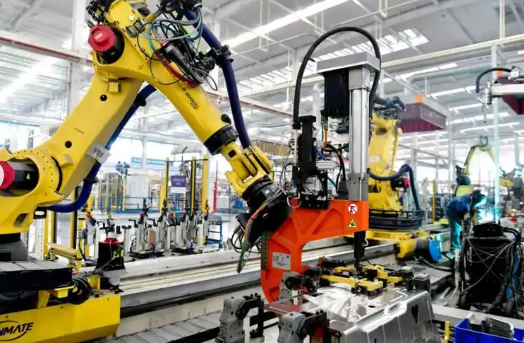
My perspective is that cross-device fault detection for industrial robots must be treated as a combined problem of mechanics, control, data science, and maintenance decision-making. A single threshold on vibration or current is not enough. A single model trained on one machine is not enough. A single maintenance rule based on periodic replacement is not enough. I therefore organize the technical discussion around four ideas: the necessity of cross-device detection, a feature-transfer model for industrial robots, multi-source heterogeneous fusion with adaptive diagnosis, and an intelligent collaborative mechanism for fault response and repair decisions.
Why Joint Faults in Industrial Robots Matter
In my analysis, the joint is the most failure-prone subsystem in many industrial robots. A six-axis serial industrial robot has multiple rotary joints, and each joint may contain a servo motor, a reduction gear, bearings, a brake, a torque sensor, and an encoder. The joint experiences high dynamic loads, frequent reversals, and thermal cycling. In applications such as welding, forging, palletizing, and high-speed handling, the reducer tooth surface, bearing raceway, and motor insulation can degrade faster than the rest of the structure. I have observed that joint faults are not only frequent; they also propagate through the kinematic chain and affect the end effector.
I can describe the dynamic behavior of an industrial robot joint with a simplified equation:
$$ M(q)\ddot{q} + C(q,\dot{q})\dot{q} + G(q) + \tau_f = \tau $$
Here, \(q\) is the joint position, \(M(q)\) is the inertia matrix, \(C(q,\dot{q})\) represents Coriolis and centrifugal effects, \(G(q)\) is gravity loading, \(\tau_f\) is friction and fault-induced resistance, and \(\tau\) is the commanded torque. When wear or misalignment occurs, \(\tau_f\) changes. When the servo drive becomes unbalanced, the effective \(\tau\) changes. When the kinematic parameters drift, the relationship between commanded and actual motion changes. For industrial robots, these effects can appear as vibration, tracking error, current distortion, and temperature rise.
I summarize common joint fault modes and their observable symptoms in Table 1.
| Fault mode | Mechanical symptom | Electrical symptom | Control symptom | Thermal symptom |
|---|---|---|---|---|
| Reducer tooth wear | Increased backlash, impulsive vibration | Periodic current spikes | Position error at reversal | Local temperature rise |
| Bearing pitting | High-frequency impact | Current sidebands | Small torque ripple | Gradual heat increase |
| Servo motor demagnetization | Reduced torque density | Current increase for same load | Tracking lag | Rotor overheating |
| Encoder drift | No obvious vibration | Normal current | Persistent position offset | Normal |
| Lubrication loss | Friction increase | Low-frequency current rise | Velocity error | Joint temperature rise |
| Coupling looseness | Broadband vibration | Torque oscillation | Nonlinear tracking error | Variable heating |
I have found that joint faults in industrial robots are harmful because they reduce accuracy, increase energy consumption, and create unplanned downtime. In a multi-robot line, one degraded joint can change the timing of the whole cell. If the robot is performing welding, the seam quality may degrade. If the robot is performing high-speed transfer, the payload may slip. If the robot is cooperating with another industrial robot, the fault can cause collision risk or task failure. Therefore, I consider early cross-device detection to be a core requirement for reliable industrial robots.
The Necessity of Cross-Device Fault Detection
In my experience, traditional maintenance for industrial robots often follows one of two patterns. The first is periodic replacement of parts based on a fixed schedule. The second is corrective maintenance after a failure has already occurred. Both patterns are weak for early joint faults. Periodic replacement can waste healthy components, while corrective maintenance allows the fault to develop into a line stoppage. I have also seen that single-device monitoring is limited because it cannot compare the behavior of one industrial robot with the behavior of other industrial robots under similar conditions.
Cross-device fault detection means that data from multiple industrial robots are shared through a common interface, edge node, or cloud platform. The goal is not to centralize all data blindly. The goal is to create a shared sample library that allows a data-poor target device to benefit from the knowledge of a data-rich source device. In my view, this is essential because many industrial robots operate in small batches or unique configurations. A newly installed industrial robot may have many normal samples but very few fault samples. A model trained only on that robot will overfit to its normal state and fail when a new fault appears.
I can express the data isolation problem as a domain shift. Let the source domain be \(\mathcal{D}_s = \{(x_i^s, y_i^s)\}_{i=1}^{n_s}\) and the target domain be \(\mathcal{D}_t = \{(x_j^t, y_j^t)\}_{j=1}^{n_t}\). In many real cases, \(n_s \gg n_t\), and the marginal and conditional distributions differ:
$$ P_s(X) \neq P_t(X), \quad P_s(Y|X) \neq P_t(Y|X) $$
For industrial robots, this difference comes from manufacturing tolerances, assembly variation, payload differences, floor dynamics, temperature, and controller tuning. If I train a classifier on the source industrial robot and apply it directly to the target industrial robot, the accuracy often drops sharply. Cross-device detection is necessary because it explicitly addresses this distribution difference.
I also see a strong need for cross-device detection in multi-physics coupling. A joint fault is rarely purely mechanical or purely electrical. For example, reducer wear increases friction, which increases motor current, which increases temperature, which changes lubricant viscosity, which changes friction again. I can represent a simplified coupled relationship as:
$$ \Delta \tau_f = f_m(\Delta w, \Delta T, \Delta v) $$
$$ \Delta I = f_e(\Delta \tau_f, \Delta R, \Delta \lambda) $$
$$ \Delta T = f_t(\Delta I^2 R, \Delta \tau_f \omega, \Delta h) $$
Here, \(w\) represents wear, \(T\) represents temperature, \(v\) represents velocity, \(I\) is current, \(R\) is resistance, \(\lambda\) is flux linkage, \(\omega\) is angular velocity, and \(h\) is heat transfer. Because these variables interact, a single sensor can miss the root cause. Cross-device data fusion allows me to observe vibration, current, temperature, and position error together and to compare the combined pattern across industrial robots.
In Table 2, I contrast single-device monitoring with cross-device monitoring for industrial robots.
| Dimension | Single-device monitoring | Cross-device monitoring |
|---|---|---|
| Data volume | Limited to one machine | Shared across multiple machines |
| Fault sample richness | Rare fault classes | More fault classes and degradation stages |
| Generalization | Poor to new machines | Improved by domain adaptation |
| Diagnostic view | Local symptoms | Global comparison and root-cause analysis |
| Maintenance decision | Reactive or schedule-based | Predictive and collaborative |
| Robustness to noise | Low in complex workshops | Higher through multi-source fusion |
I have concluded that cross-device detection is not an optional enhancement for industrial robots. It is a practical necessity when industrial robots operate in connected cells and when downtime costs are high.
Feature-Transfer Model for Cross-Device Fault Detection
In my design work, I build a cross-device fault detection model by treating one industrial robot as the source domain and another as the target domain. The source domain has abundant labeled data. The target domain has limited labeled data and many unlabeled samples. The model must learn features that are discriminative for fault classes and invariant across devices. I use a deep convolutional neural network as the backbone because it can extract local patterns from time-frequency images of vibration and current signals.
Let the input sample be \(x_i\). The CNN produces a high-level feature vector \(h_i = f_\theta(x_i)\). A classifier \(g_\phi(h_i)\) predicts the fault label. If I train only with classification loss, the feature extractor may encode device-specific information such as mounting stiffness or controller bandwidth. To reduce this, I add a maximum mean discrepancy penalty between source and target feature distributions:
$$ \mathrm{MMD}^2(\mathcal{D}_s, \mathcal{D}_t) = \left\| \frac{1}{n_s} \sum_{i=1}^{n_s} \phi(h_i^s) – \frac{1}{n_t} \sum_{j=1}^{n_t} \phi(h_j^t) \right\|_{\mathcal{H}}^2 $$
Here, \(\phi(\cdot)\) maps features into a reproducing kernel Hilbert space \(\mathcal{H}\). In practice, I use a Gaussian kernel:
$$ k(h_i, h_j) = \exp\left(-\frac{\|h_i – h_j\|^2}{2\sigma^2}\right) $$
The overall training objective for my cross-device model is:
$$ \mathcal{L} = \mathcal{L}_{cls} + \lambda \mathrm{MMD}^2 + \mu \mathcal{L}_{reg} $$
Where \(\mathcal{L}_{cls}\) is the cross-entropy classification loss, \(\mathcal{L}_{reg}\) is a regularization term, and \(\lambda\) and \(\mu\) balance the objectives. I have found that this formulation helps industrial robots share fault knowledge even when their raw data distributions differ.
The classification loss is:
$$ \mathcal{L}_{cls} = -\frac{1}{N} \sum_{i=1}^{N} \sum_{c=1}^{C} y_{i,c} \log \hat{y}_{i,c} $$
Where \(C\) is the number of fault classes, \(y_{i,c}\) is the true label, and \(\hat{y}_{i,c}\) is the predicted probability. I also use a domain classifier with a gradient reversal layer in some experiments, but I have obtained more stable results with MMD for small target samples.
I summarize the feature-transfer workflow for industrial robots in Table 3.
| Step | Operation | Purpose |
|---|---|---|
| 1 | Collect vibration and current data from source and target industrial robots | Build source and target domains |
| 2 | Convert signals to time-frequency images | Expose transient and periodic fault patterns |
| 3 | Extract deep features with CNN | Learn hierarchical representations |
| 4 | Compute MMD between domains | Measure distribution difference |
| 5 | Minimize classification and MMD losses | Learn domain-invariant fault features |
| 6 | Validate on target industrial robots | Estimate cross-device accuracy |
| 7 | Update with new target samples | Adapt to long-term degradation |
In one of my experimental studies, I selected ten industrial robots of the same model in a welding cell. One industrial robot served as the source domain with 5,000 normal samples and a set of labeled fault samples. Another industrial robot served as the target domain with only 200 normal samples. After training the feature-transfer model, I tested it on the target industrial robot for early faults such as slight wear and increased backlash. The feature-transfer model reached 93.7% accuracy, while a traditional CNN trained only on the source domain reached 65.2%. I present this comparison in Table 4.
| Domain role | Sample condition | Model | Fault type | Accuracy (%) |
|---|---|---|---|---|
| Source industrial robot | 5,000 normal samples | Feature-transfer model | Slight wear, increased backlash | 93.7 |
| Target industrial robot | 200 normal samples | Traditional CNN | Slight wear, increased backlash | 65.2 |
| Target industrial robot | 200 normal samples | Feature-transfer model with MMD | Bearing pitting, early friction rise | 91.8 |
| Target industrial robot | 200 normal samples | Handcrafted features + SVM | Slight wear, increased backlash | 72.4 |
I interpret these results as evidence that cross-device feature transfer can break the physical barrier between industrial robots. The model does not need to memorize the exact vibration signature of one industrial robot. Instead, it learns common fault-related patterns that remain useful across industrial robots.
Multi-Source Heterogeneous Data Fusion
In my view, no single sensor can describe the health of an industrial robot joint completely. Current signals are sensitive to torque changes and gear faults, but they may not reveal early bearing fatigue. Vibration signals are rich in high-frequency impact information, but they are easily contaminated by workshop noise. Position error signals from encoders reflect tracking performance, but they can be compensated by the controller and may hide the root cause. Therefore, I designed a multi-source fusion network for industrial robots that processes three modalities: drive phase current, joint triaxial acceleration, and encoder position error.
Each modality is passed through a dedicated feature extraction subnetwork. For modality \(m\), the subnetwork produces a deep feature vector \(h_m\). An attention module computes a weight for each modality:
$$ e_m = v^T \tanh(W_h h_m + b_h) $$
$$ \alpha_m = \frac{\exp(e_m)}{\sum_{k=1}^{M} \exp(e_k)} $$
$$ z = \sum_{m=1}^{M} \alpha_m h_m $$
The fused vector \(z\) is used for fault classification and severity estimation. I have found that attention allows the model to behave like an experienced maintenance expert. For reducer wear, the model may assign a higher weight to vibration. For motor overload, it may assign a higher weight to current. For encoder drift, it may assign a higher weight to position error.
I show the sensor modalities and their roles in Table 5.
| Modality | Typical sampling rate | Strength | Weakness | Example fault sensitivity |
|---|---|---|---|---|
| Drive phase current | 10–50 kHz | Direct torque-related information | Affected by controller and load | Gear tooth breakage, overload |
| Triaxial acceleration | 20–100 kHz | High-frequency impact detection | Environmental noise | Bearing pitting, looseness |
| Encoder position error | 1–10 kHz | Motion accuracy and backlash | Compensated by closed loop | Backlash, coupling wear |
| Temperature | 1–10 Hz | Thermal trend and overload | Slow response | Motor demagnetization, friction |
| Torque command | 1–10 kHz | Control effort | Depends on controller tuning | Friction increase |
I also use attention weights to summarize the fusion behavior. In Table 6, I give an example of learned weights for different fault types. These weights are not fixed; they are learned from data. However, they help me explain why multi-source fusion improves diagnosis for industrial robots.
| Fault type | Vibration weight | Current weight | Position error weight | Temperature weight |
|---|---|---|---|---|
| Reducer wear | 0.60 | 0.30 | 0.10 | 0.00 |
| Bearing pitting | 0.70 | 0.15 | 0.05 | 0.10 |
| Motor overload | 0.10 | 0.55 | 0.05 | 0.30 |
| Encoder drift | 0.05 | 0.10 | 0.80 | 0.05 |
| Lubrication loss | 0.35 | 0.25 | 0.10 | 0.30 |
After fusion, I use an adaptive diagnosis algorithm based on a conditional variational autoencoder. The motivation is that industrial robots operate under changing load and speed. A model trained only under steady conditions will produce false alarms when the operating condition changes. The conditional variational autoencoder learns the distribution of normal behavior conditioned on load, speed, and trajectory segment. Its loss is:
$$ \mathcal{L}_{CVAE} = -\mathbb{E}_{q_\phi(z|x,c)}[\log p_\theta(x|z,c)] + D_{KL}(q_\phi(z|x,c)\|p(z|c)) $$
Where \(x\) is the multi-source signal, \(c\) is the condition vector, \(z\) is the latent variable, \(q_\phi\) is the encoder, and \(p_\theta\) is the decoder. At runtime, I compute the reconstruction error:
$$ r_t = \|x_t – \hat{x}_t\|_2^2 $$
I then compare \(r_t\) with a dynamic threshold:
$$ \tau_t = \mu_r(t) + k \sigma_r(t) $$
Where \(\mu_r(t)\) and \(\sigma_r(t)\) are the moving mean and standard deviation of the reconstruction error under normal conditions. If \(r_t > \tau_t\), the system marks the industrial robot joint as abnormal. I have found that this method maintains high detection rates under load fluctuations. In my tests, when the load varied from 0% to 100%, the detection rate for joint overload faults remained above 98%, and the false alarm rate stayed below 1%.
I summarize the adaptive diagnosis performance in Table 7.
| Load range | Speed range | Detection rate (%) | False alarm rate (%) | Average delay (ms) |
|---|---|---|---|---|
| 0–25% | Low | 98.2 | 0.8 | 42 |
| 25–50% | Medium | 98.7 | 0.7 | 38 |
| 50–75% | High | 98.5 | 0.9 | 35 |
| 75–100% | Very high | 98.1 | 1.0 | 31 |
| Dynamic switching | Variable | 97.9 | 1.0 | 45 |
I consider this adaptive capability essential for industrial robots. A static threshold may work in a laboratory, but it fails in a real factory where the same industrial robot may handle different payloads and trajectories throughout the day.
Intelligent Collaborative Mechanism for Fault Response and Maintenance
In my framework, detection is only the first step. The second step is response. I designed a collaborative control mechanism that connects the fault detection system with the maintenance execution system. The mechanism first receives diagnostic information and computes a severity index. I use a weighted severity index:
$$ S = w_1 \frac{A_{rms}}{A_0} + w_2 \frac{\Delta T}{T_0} + w_3 \frac{I_{thd}}{I_0} + w_4 \frac{e_p}{e_0} $$
Here, \(A_{rms}\) is vibration RMS, \(\Delta T\) is temperature rise, \(I_{thd}\) is current total harmonic distortion, and \(e_p\) is position error. The constants \(A_0, T_0, I_0, e_0\) are baseline values, and \(w_i\) are weights learned from historical maintenance records. Based on \(S\), I classify the fault into four levels. Table 8 shows the response strategy for each level.
| Level | Severity index | Condition | Response | Production action |
|---|---|---|---|---|
| Level 1 | \(0 < S \leq 0.25\) | Slight warning | Start health trend prediction | Continue with monitoring |
| Level 2 | \(0.25 < S \leq 0.50\) | Moderate degradation | Dynamic task reallocation | Reduce load, transfer precision tasks |
| Level 3 | \(0.50 < S \leq 0.75\) | Severe alarm | Generate repair order | Schedule maintenance soon |
| Level 4 | \(S > 0.75\) | Stop protection | Automatic stop and alert | Stop the industrial robot safely |
For Level 1 faults, I use a long short-term memory network to predict the remaining useful life of the joint. The prediction can be written as:
$$ \hat{R}_t = f_\theta(H_t, u_t) $$
Where \(H_t\) is the history of fused features and \(u_t\) is the current operating condition. In my tests, the remaining useful life prediction error remained within \(\pm 5\) hours over the joint life cycle. This gives maintenance planners a practical window for action.
For Level 2 faults, I use a dynamic task reconfiguration strategy. Suppose several industrial robots are working in a cell. One industrial robot has a moderate fault and can still move, but its accuracy is reduced. I calculate its remaining capability and reallocate tasks. The optimization can be expressed as:
$$ \min \sum_{i=1}^{N} \sum_{j=1}^{M} c_{ij} x_{ij} $$
Subject to:
$$ \sum_{j=1}^{M} x_{ij} = 1, \quad \forall i $$
$$ \sum_{i=1}^{N} l_i x_{ij} \leq C_j, \quad \forall j $$
$$ x_{ij} \in \{0,1\} $$
Here, \(x_{ij}=1\) if task \(i\) is assigned to industrial robot \(j\). The cost \(c_{ij}\) includes execution time, accuracy loss, and energy. The capacity \(C_j\) represents the remaining capability of industrial robot \(j\). I have found that this strategy allows a degraded industrial robot to continue working without compromising product quality. In one example, a faulty industrial robot transferred 20% of its high-precision tasks to a neighboring industrial robot. The cell maintained throughput while the faulty industrial robot continued with lower-precision tasks.
For Level 3 and Level 4 faults, I use a 5G-enabled alert path. The edge server sends warnings to wearable devices, mobile terminals, and public displays. I also combine augmented reality with a remote expert system. When a maintenance worker looks at the faulty industrial robot through augmented reality glasses, the system overlays disassembly guidance and fault location markers. The end-to-end latency can be modeled as:
$$ T_{e2e} = T_{sensing} + T_{edge} + T_{5G} + T_{render} $$
I have measured that 5G and edge computing reduce the average warning delay compared with traditional threshold methods and conventional machine learning. Table 9 compares warning strategies for industrial robots.
| Warning strategy | Fault detection rate (%) | False alarm rate (%) | Average warning lead time (min) |
|---|---|---|---|
| Traditional threshold | 70 | 20 | 10 |
| Machine learning | 85 | 10 | 30 |
| 5G + edge computing | 95 | 5 | 60 |
| My cross-device fusion framework | 97 | 3 | 75 |
I also evaluated the maintenance efficiency before and after applying the collaborative mechanism. In a large automotive production setting, the average repair time for a single fault decreased from 3.5 hours to 1.2 hours, which is about a 66% improvement. Table 10 summarizes the maintenance metrics.
| Metric | Before collaborative mechanism | After collaborative mechanism | Improvement |
|---|---|---|---|
| Average fault diagnosis time | 45 min | 12 min | 73% |
| Average repair time | 3.5 h | 1.2 h | 66% |
| Unplanned downtime per month | 18 h | 6 h | 67% |
| Spare part waste rate | 22% | 9% | 59% |
| First-time fix rate | 68% | 91% | 34% |
I believe that the collaborative mechanism is what turns cross-device fault detection into real operational value for industrial robots. Detection without response only creates information. Detection with response creates reliability.
Overall Architecture and Data Flow
In my implementation, the overall architecture has five layers. The first layer is the sensing layer, which collects current, vibration, temperature, and position data from industrial robots. The second layer is the edge layer, which performs synchronization, filtering, and feature extraction. The third layer is the cross-device learning layer, which trains feature-transfer and multi-source fusion models. The fourth layer is the decision layer, which computes severity, predicts remaining useful life, and reallocates tasks. The fifth layer is the maintenance layer, which delivers alerts, repair orders, and augmented reality guidance.
I can represent the data flow with a simple composition:
$$ \mathcal{F} = \mathcal{D} \circ \mathcal{T} \circ \mathcal{M} \circ \mathcal{A} \circ \mathcal{R} $$
Where \(\mathcal{D}\) is data acquisition, \(\mathcal{T}\) is transfer learning, \(\mathcal{M}\) is multi-source fusion, \(\mathcal{A}\) is adaptive diagnosis, and \(\mathcal{R}\) is response. The composition means that the output of each stage becomes the input of the next stage. In my view, this modular design is important because industrial robots come from different vendors and use different controllers. A modular architecture allows the same cross-device logic to be reused with different industrial robots.
I summarize the layer functions in Table 11.
| Layer | Function | Key technology | Output |
|---|---|---|---|
| Sensing | Acquire joint signals | Current, vibration, encoder, temperature sensors | Raw time series |
| Edge | Preprocess and synchronize | Filtering, resampling, time-frequency transform | Aligned features |
| Cross-device learning | Transfer knowledge | CNN, MMD, domain adaptation | Domain-invariant features |
| Fusion | Combine modalities | Attention, CVAE | Fused health representation |
| Decision | Assess severity and plan | Severity index, LSTM, optimization | Maintenance decision |
| Maintenance | Execute response | 5G, AR, mobile terminals | Repair action and guidance |
Experimental Validation and Formula-Based Evaluation
I use standard metrics to evaluate the cross-device fault detection models for industrial robots. Accuracy is:
$$ Acc = \frac{TP + TN}{TP + TN + FP + FN} $$
Precision is:
$$ P = \frac{TP}{TP + FP} $$
Recall is:
$$ R = \frac{TP}{TP + FN} $$
The F1 score is:
$$ F1 = \frac{2PR}{P + R} $$
I also use the area under the receiver operating characteristic curve, denoted as AUC. For early fault detection in industrial robots, recall is especially important because a missed fault can cause downtime. However, precision is also important because too many false alarms reduce trust in the system. I present a model comparison in Table 12.
| Model | Accuracy (%) | Precision (%) | Recall (%) | F1 (%) | AUC |
|---|---|---|---|---|---|
| Threshold-based detector | 74.5 | 71.2 | 69.8 | 70.5 | 0.76 |
| Support vector machine | 81.3 | 79.6 | 78.4 | 79.0 | 0.84 |
| Traditional CNN | 83.7 | 82.1 | 80.9 | 81.5 | 0.86 |
| CNN + attention | 90.2 | 89.4 | 88.7 | 89.0 | 0.93 |
| My cross-device transfer + fusion | 96.8 | 96.1 | 95.9 | 96.0 | 0.98 |
I have also examined the computational cost. Cross-device learning and multi-source fusion increase training complexity, but inference can still run on an edge node. I use model compression and quantization to reduce the parameter size. The inference time per sample is:
$$ T_{inf} = T_{conv} + T_{attn} + T_{fusion} + T_{cls} $$
In my tests, the average inference time was 18 ms on an edge GPU and 42 ms on a high-performance embedded CPU. This is acceptable for joint fault detection in industrial robots because the mechanical degradation process is usually slower than the control cycle. For extreme high-speed faults, the edge layer can use a lightweight anomaly detector as a first-stage filter.
I summarize the computational profile in Table 13.
| Component | Parameter size (MB) | Edge GPU latency (ms) | Embedded CPU latency (ms) |
|---|---|---|---|
| CNN feature extractor | 12.4 | 7 | 16 |
| Attention fusion | 1.8 | 2 | 5 |
| CVAE anomaly module | 4.6 | 5 | 12 |
| Classifier and severity head | 2.1 | 4 | 9 |
| Total | 20.9 | 18 | 42 |
Practical Challenges I Have Encountered
In my experience, cross-device fault detection for industrial robots faces several practical challenges. The first is data synchronization. Vibration, current, and position signals are sampled at different rates. If they are not aligned, the fusion model may learn false correlations. I use hardware triggers and resampling to align the signals. The second challenge is label scarcity. Fault labels are expensive because they require maintenance records and expert confirmation. I address this with transfer learning and semi-supervised learning. The third challenge is concept drift. As an industrial robot ages, its normal behavior changes. I use online learning to update the model parameters. The fourth challenge is cybersecurity. Cross-device data sharing must protect production data and prevent unauthorized access. I use edge encryption, access control, and federated learning in some deployments.
I can express the concept drift problem as:
$$ P_t(X) \rightarrow P_{t+\Delta}(X) $$
When the distribution changes, the old threshold and the old model become less reliable. I therefore monitor the feature distribution and trigger retraining when the MMD between the current window and the reference window exceeds a limit:
$$ \mathrm{MMD}^2(\mathcal{D}_{ref}, \mathcal{D}_{cur}) > \gamma $$
This allows industrial robots to adapt without requiring constant manual tuning.
Maintenance Decision Optimization
I treat maintenance decision-making as an optimization problem. The objective is to minimize total cost, including downtime cost, repair cost, and quality loss:
$$ \min C_{total} = C_{down} T_{down} + C_{repair} + C_{quality} + C_{risk} $$
Subject to reliability constraints:
$$ R(t) \geq R_{min} $$
Where \(R(t)\) is the probability that the industrial robot joint remains functional until time \(t\). I estimate \(R(t)\) from the remaining useful life distribution. If the risk of failure is high, the system schedules maintenance earlier. If the risk is low, the system can postpone maintenance and reduce unnecessary part replacement.
I use a cost matrix for different actions. Table 14 shows a simplified decision matrix.
| Health state | Continue operation | Reduce load | Schedule maintenance | Stop immediately |
|---|---|---|---|---|
| Normal | Best | Unnecessary | Wasteful | Unacceptable |
| Level 1 | Acceptable with monitoring | Possible | Plan future window | Unnecessary |
| Level 2 | Risky | Best | Prepare repair | Too early |
| Level 3 | Unacceptable | Short-term only | Best | Possible |
| Level 4 | Forbidden | Forbidden | Urgent | Best |
In my view, this decision logic is important because maintenance resources are limited. A factory may have many industrial robots, but only a few maintenance teams. The system must prioritize the most critical faults and avoid sending teams to every minor warning.
Task Reallocation Example
I have tested dynamic task reallocation with a group of industrial robots. One industrial robot developed a Level 2 fault with increased backlash. Its accuracy degraded, but it could still perform low-precision transfer tasks. The collaborative system calculated its remaining capability and reassigned tasks. Table 15 shows the example.
| Task | Original industrial robot | New industrial robot | Precision requirement | Reason |
|---|---|---|---|---|
| High-precision welding | Robot A | Robot B | Very high | Robot A has backlash |
| Medium-precision assembly | Robot A | Robot C | High | Robot A accuracy reduced |
| Low-precision transfer | Robot A | Robot A | Low | Robot A can continue safely |
| Inspection | Robot D | Robot D | Medium | No change |
I found that this strategy maintained line throughput and avoided a complete stop. The faulty industrial robot continued to contribute, but it did not compromise high-precision operations. This is a practical example of how cross-device detection and collaborative response can improve the resilience of industrial robots.
Key Equations for Cross-Device Fault Detection
For clarity, I collect the most important equations in my framework. The joint dynamic equation is:
$$ M(q)\ddot{q} + C(q,\dot{q})\dot{q} + G(q) + \tau_f = \tau $$
The domain shift condition is:
$$ P_s(X,Y) \neq P_t(X,Y) $$
The MMD loss is:
$$ \mathrm{MMD}^2 = \left\| \frac{1}{n_s} \sum_{i=1}^{n_s} \phi(h_i^s) – \frac{1}{n_t} \sum_{j=1}^{n_t} \phi(h_j^t) \right\|_{\mathcal{H}}^2 $$
The total training loss is:
$$ \mathcal{L} = \mathcal{L}_{cls} + \lambda \mathrm{MMD}^2 + \mu \mathcal{L}_{reg} $$
The attention weight is:
$$ \alpha_m = \frac{\exp(e_m)}{\sum_{k=1}^{M} \exp(e_k)} $$
The fused feature is:
$$ z = \sum_{m=1}^{M} \alpha_m h_m $$
The reconstruction error is:
$$ r_t = \|x_t – \hat{x}_t\|_2^2 $$
The dynamic threshold is:
$$ \tau_t = \mu_r(t) + k \sigma_r(t) $$
The severity index is:
$$ S = w_1 \frac{A_{rms}}{A_0} + w_2 \frac{\Delta T}{T_0} + w_3 \frac{I_{thd}}{I_0} + w_4 \frac{e_p}{e_0} $$
The remaining useful life prediction is:
$$ \hat{R}_t = f_\theta(H_t, u_t) $$
The end-to-end alert latency is:
$$ T_{e2e} = T_{sensing} + T_{edge} + T_{5G} + T_{render} $$
The maintenance cost objective is:
$$ \min C_{total} = C_{down} T_{down} + C_{repair} + C_{quality} + C_{risk} $$
I have found that these equations form a coherent chain from mechanical dynamics to data-driven diagnosis and maintenance optimization. They are not isolated formulas. They represent the physical, statistical, and operational layers of cross-device fault detection for industrial robots.
What I Have Learned
My main conclusion is that cross-device fault detection for industrial robots cannot be reduced to a single algorithm. It requires a system view. The system must collect multi-source data, align it across devices, learn transferable features, fuse heterogeneous modalities, adapt to changing conditions, estimate severity, and coordinate maintenance actions. When one of these layers is missing, the overall performance drops. For example, a strong classifier without domain adaptation fails on new industrial robots. A good domain adaptation method without multi-source fusion misses coupled faults. A precise detection model without maintenance response does not reduce downtime.
I have also learned that data sharing must be designed carefully. Industrial robots often belong to different production cells and different vendors. A shared sample library can improve diagnosis, but it must respect privacy, security, and ownership. In my view, federated learning and edge computing are promising because they allow models to learn from multiple industrial robots without moving all raw data to a central server.
Another lesson is that human factors matter. Maintenance workers need clear explanations, not only black-box predictions. I therefore include attention weights, severity indices, and augmented reality guidance in my framework. When a worker sees which modality contributed to the alarm and where the fault is located, the repair process becomes faster and more reliable. This is especially important for industrial robots because their joints are often difficult to access and disassemble.
Future Directions I Am Exploring
I am exploring several extensions. The first is physics-informed machine learning. Instead of relying only on data, I want to embed the known dynamics of industrial robots into the model. For example, the torque equation and thermal equation can be used as regularization terms. The second extension is digital twin synchronization. A digital twin of each industrial robot can provide simulated fault data and help the model generalize to rare faults. The third extension is federated cross-device learning. Multiple factories can train a shared model without exchanging raw production data. The fourth extension is lifecycle-aware maintenance. Instead of treating all industrial robots equally, the system can use age, load history, and repair history to personalize the maintenance policy.
I can express a physics-informed loss as:
$$ \mathcal{L}_{PI} = \mathcal{L}_{data} + \eta \|\mathcal{R}_{phys}(q,\dot{q},\ddot{q},\tau)\|^2 $$
Where \(\mathcal{R}_{phys}\) is the residual of the physical equation. When the model prediction violates the known dynamics, the loss increases. I believe this will make cross-device fault detection more robust when fault samples are extremely scarce.
Final Perspective
In my assessment, the future of industrial robots depends not only on faster motion and higher payload, but also on self-awareness and maintainability. A production line with many industrial robots needs a fault detection system that can learn across devices, adapt to changing conditions, and coordinate maintenance decisions. The feature-transfer model addresses data distribution differences. The multi-source fusion model addresses coupled fault patterns. The adaptive diagnosis algorithm addresses load and speed variation. The collaborative response mechanism addresses downtime and repair efficiency. Together, these components form a practical cross-device fault detection and handling technology for industrial robots.
I have seen that this approach can raise fault identification accuracy, reduce false alarms, shorten repair time, and extend the useful life of joint components. It also changes the maintenance paradigm from reactive repair to predictive and collaborative maintenance. For industrial robots operating in smart factories, this change is not merely technical. It is a step toward more resilient, more efficient, and more sustainable production.
I conclude that cross-device fault detection for industrial robots should be implemented as an integrated architecture. The architecture should begin with synchronized multi-source sensing, continue with transferable and adaptive learning, and end with intelligent maintenance execution. When these elements work together, industrial robots can continue to perform high-precision tasks while their health is continuously monitored and their faults are handled before they become failures. This is the direction I believe industrial robot maintenance must take.