
In the field of precision mechanical transmission, strain wave gear drives, also known as harmonic drives, have garnered significant attention due to their unique advantages such as high reduction ratios, compact design, and zero-backlash operation. As a researcher focused on gear mechanics, I have long been intrigued by the complex kinematics of these systems, particularly the concept of contact ratio. The contact ratio is a critical parameter that influences the continuity of motion, load distribution, and overall smoothness of operation. Unlike conventional rigid gear systems, strain wave gear drives involve elastic deformation of the flexspline, which complicates the analysis of meshing behavior. In this article, I will present a comprehensive methodology for computing the contact ratio of strain wave gear drives, drawing upon kinematic geometry and fundamental theorems of gearing. This approach is designed to be universal, applicable to various tooth profiles, and relies heavily on mathematical derivations, including equations and tables, to elucidate the process. Throughout this discussion, the term “strain wave gear” will be emphasized to underscore the focus on this specific transmission technology.
The contact ratio in gear systems traditionally refers to the average number of tooth pairs in contact during operation, ensuring smooth power transmission. For strain wave gear drives, however, this definition must be adapted to account for the elastic conjugate motion between the flexspline and the circular spline. Based on my research, I define the contact ratio for strain wave gear drives as the ratio of the meshing angle between the teeth of the flexspline and the circular spline to the central angle corresponding to a single pitch of the circular spline. This definition captures the essence of simultaneous tooth engagement in these deformable systems. Mathematically, it can be expressed as:
$$ \epsilon = \frac{N (\theta + \theta’) Z}{360} = \frac{N \Phi Z}{360} $$
where \( \epsilon \) is the contact ratio, \( N \) is the wave number (typically 2 for common strain wave gear drives), \( \Phi = \theta + \theta’ \) is the total meshing angle for a single tooth, with \( \theta \) and \( \theta’ \) representing the engagement and disengagement angles, respectively, and \( Z \) is the number of teeth on the circular spline (or flexspline). This formula provides a theoretical basis, but in practice, factors like load application can shift meshing points, altering the actual contact interval. Thus, developing a robust computational method is essential for evaluating new tooth profiles and optimizing strain wave gear performance.
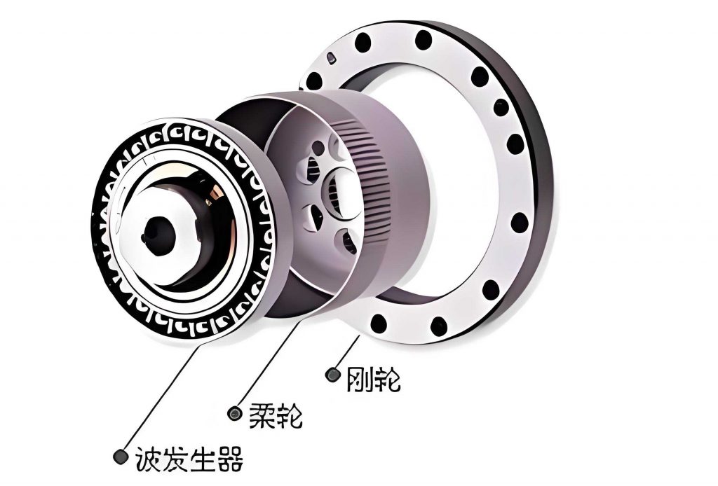
To compute the contact ratio, I base my approach on kinematic geometry and Willis theorem, which states that the common normal at the point of contact between two gear tooth profiles must pass through the relative instantaneous center of the two profiles. This theorem is pivotal for analyzing conjugate motion in strain wave gear drives. The process involves several steps: first, deriving the equation for the instantaneous center curve of the flexspline tooth relative to a fixed frame; second, determining the relative instantaneous center curve between the flexspline and circular spline; and finally, using Willis theorem to calculate the meshing angle \( \Phi \). This methodology is independent of tooth shape, making it versatile for various strain wave gear designs.
In strain wave gear drives, the motion is driven by a wave generator, often a cam, that deforms the flexspline into an elliptical shape. I assume a fixed wave generator, with the flexspline as the input and the circular spline as the output. The wave generator’s profile significantly influences the kinematics. A common design uses a cosine cam profile, which can be described in polar coordinates. Let \( \sigma = [O; \mathbf{e}_1, \mathbf{e}_2] \) be the fixed frame attached to the wave generator, where the \( \mathbf{e}_2 \)-axis aligns with the cam’s major axis. The cam profile is given by:
$$ \rho_H = r_c + \omega_0 \cos 2\psi $$
where \( \rho_H \) is the polar radius of the ellipse, \( r_c \) is the radius of the neutral circle of the undeformed flexspline, \( \omega_0 \) is the maximum radial deformation of the flexspline midline, and \( \psi \) is the angle between the polar radius and the \( \mathbf{e}_2 \)-axis. In the fixed frame \( \sigma \), the coordinates of a point on the cam profile are:
$$ x_{OF} = \rho_H \sin \psi, \quad y_{OF} = \rho_H \cos \psi $$
These equations form the foundation for analyzing the flexspline’s motion. The flexspline tooth’s instantaneous center of rotation, denoted as point \( O_1 \), varies due to the elastic deformation. To find its trajectory, I consider the velocity of \( O_1 \) relative to the fixed frame. Since \( O_1 \) is attached to the flexspline tooth frame \( \sigma^{(F)} = [O_F; \mathbf{e}_1^{(F)}, \mathbf{e}_2^{(F)}] \), where \( \mathbf{e}_2^{(F)} \) aligns with the tooth symmetry line, its coordinates in \( \sigma^{(F)} \) are constants. By applying kinematic relations and setting the velocity to zero, I derive the coordinates of \( O_1 \) in \( \sigma^{(F)} \):
$$ x_1^{(F)} = 0, \quad x_2^{(F)} = -\rho $$
Here, \( \rho \) is the radius of curvature of the cam ellipse at point \( O_F \), calculated using standard curvature formulas from differential geometry:
$$ \rho = \frac{(\dot{x}_{OF}^2 + \dot{y}_{OF}^2)^{3/2}}{\dot{x}_{OF} \ddot{y}_{OF} – \ddot{x}_{OF} \dot{y}_{OF}} $$
where dots denote derivatives with respect to \( \psi \). Transforming these coordinates to the fixed frame \( \sigma \), I obtain:
$$ x_{O1} = x_{OF} – \rho \sin(\psi + \mu), \quad y_{O1} = y_{OF} – \rho \cos(\psi + \mu) $$
In this equation, \( \mu \) is the angle between \( \mathbf{e}_2^{(F)} \) and the line connecting the origin \( O \) to \( O_F \), which depends on the cam profile. Using software like MATLAB, the trajectory of \( O_1 \) can be simulated, often resembling a astroid-like curve, highlighting the complex motion in strain wave gear drives.
Next, I determine the relative instantaneous center curve between the flexspline and circular spline. Let \( \sigma^{(2)} = [O_2; \mathbf{e}_1^{(2)}, \mathbf{e}_2^{(2)}] \) be the frame attached to the circular spline, with \( O_2 \) as its rotation center (coinciding with the fixed origin \( O \) in the initial position). The relative instantaneous center \( P \) is the point where the two bodies have no relative velocity. Based on kinematic theory, the coordinates of \( P \) in the fixed frame \( \sigma \) are derived from the angular velocities of the flexspline and circular spline. Assuming the wave generator is fixed, the angular velocities are:
$$ \omega_1 = \frac{d\theta}{d\psi} \cdot \frac{d\psi}{dt}, \quad \omega_2 = \left(1 + \frac{d\mu}{d\psi}\right) \cdot \frac{d\psi}{dt} $$
where \( \theta \) is the rotation angle of the circular spline from its initial position, and \( \frac{d\mu}{d\psi} \) is computed from the cam profile geometry. The relative instantaneous center coordinates are:
$$ x_P = \frac{\omega_2}{\omega_2 – \omega_1} x_{O1}, \quad y_P = \frac{\omega_2}{\omega_2 – \omega_1} y_{O1} $$
This equation shows that the relative instantaneous center depends solely on the wave generator’s shape and the kinematics, not on the tooth profiles, reinforcing the generality of this method for strain wave gear analysis.
With the relative instantaneous center curve established, I apply Willis theorem to compute the meshing angle \( \Phi \). Consider a point \( M \) on the circular spline tooth profile where contact occurs. In the circular spline frame \( \sigma^{(2)} \), let the left tooth profile be described by \( y_R = f(x_R) \). The normal line at point \( M(x_0, y_0) \) is given by:
$$ y_R = -\frac{1}{f'(x_0)} (x_R – x_0) + y_0 $$
Transforming this normal to the fixed frame \( \sigma \) using a rotation matrix with angle \( \theta \), the equation becomes:
$$ y = -\tan \theta \cdot x – y_R \sin \theta + y_R \cos \theta $$
According to Willis theorem, this normal must pass through the relative instantaneous center \( P(x_P, y_P) \). Substituting \( P \)’s coordinates into the normal equation allows solving for \( \theta \), which represents the rotation angle of the circular spline at which contact occurs. By identifying the limits of contact—such as the engagement and disengagement points on the tooth profile—I can determine \( \theta \) and \( \theta’ \), and thus \( \Phi \). For instance, in a single-circular-arc tooth profile, the contact points range from the addendum to the dedendum, defining the meshing interval.
To illustrate the computational process, I provide a numerical example using a single-circular-arc tooth profile for the circular spline in a strain wave gear drive. The key parameters are summarized in the table below:
| Parameter | Symbol | Value |
|---|---|---|
| Module | \( m \) | 0.5 mm |
| Circular spline teeth | \( Z_G \) | 152 |
| Flexspline teeth | \( Z_F \) | 150 |
| Wave number | \( N \) | 2 |
| Maximum radial deformation | \( \omega_0 \) | Derived from design |
| Tooth profile radius | \( \rho_\alpha \) | Based on arc geometry |
The circular spline tooth profile equation in frame \( \sigma^{(2)} \) is:
$$ x_g = L – \rho_\alpha \cos \alpha + C, \quad y_g = r_R – \rho_\alpha \sin \alpha $$
where \( L \) is the distance between symmetry lines of convex and concave teeth, \( r_R \) is the pitch radius of the circular spline, \( \rho_\alpha \) is the radius of the circular arc, \( \alpha \) is the profile angle, and \( C \) is the center offset of the arc. The engagement limits are defined by points \( A \) (addendum) and \( B \) (dedendum). Using the derived equations, I compute the normal lines at these points, substitute the relative instantaneous center coordinates, and solve for \( \theta \) and \( \theta’ \). For this example, the calculation yields:
$$ \Phi = 53.864^\circ, \quad \epsilon = \frac{2 \times 53.864 \times 152}{360} \approx 45.486 $$
This result demonstrates that strain wave gear drives exhibit a contact ratio significantly higher than that of conventional gears—often by an order of magnitude—which explains their superior load-bearing capacity and smooth operation. The computation can be implemented in programming languages like C or Python for efficiency.
The methodology I have described offers several advantages for strain wave gear analysis. Firstly, it is grounded in well-established kinematic principles, ensuring theoretical rigor. Secondly, by decoupling the tooth profile from the instantaneous center derivation, it applies universally to various tooth shapes, whether involute, circular-arc, or novel profiles. This is particularly valuable for designing new strain wave gear configurations where evaluating meshing performance is crucial. However, it is important to note that this approach computes the theoretical contact ratio; practical factors like manufacturing tolerances, load distribution, and material elasticity may affect actual meshing. Future work could integrate finite element analysis to refine these calculations.
In conclusion, computing the contact ratio for strain wave gear drives requires a specialized approach due to their elastic deformation characteristics. Through this article, I have detailed a method based on instantaneous center curves and Willis theorem, which provides a universal framework for different tooth profiles. The high contact ratio calculated—exemplified by the numerical example—underscores the operational advantages of strain wave gear drives, including enhanced durability and transmission stability. As research in this field progresses, this computational technique will serve as a foundational tool for optimizing strain wave gear designs and advancing their applications in robotics, aerospace, and precision machinery. By repeatedly emphasizing “strain wave gear,” I highlight the focus on this innovative transmission technology, which continues to evolve through such analytical efforts.