
In my research and engineering practice on flexible avionics assembly, I concentrate on the high-precision positioning and error compensation of industrial robots. Avionics systems integrate many delicate components, including printed circuit boards, wire harness connectors, and airborne modules. These components require precise insertion and mating operations. Flexible assembly lines increasingly rely on industrial robots because they offer programmability, reconfigurability, and repeatability. However, the absolute positioning accuracy of general-purpose industrial robots is often insufficient for avionics-grade tolerances. Therefore, I develop a systematic method that combines modified Denavit-Hartenberg modeling, laser tracker measurement, improved particle filtering, and automatic error compensation. The goal is to enable industrial robots to achieve sub-millimeter positioning accuracy and to support reliable precision assembly in flexible avionics production.
The core problem is that industrial robots accumulate errors from multiple sources. Geometric parameter errors arise from manufacturing and assembly deviations in link lengths, joint offsets, and twist angles. Non-geometric errors arise from joint flexibility, gear backlash, transmission friction, and link bending. Environmental errors arise from temperature fluctuations, measurement noise, and controller quantization. These errors interact in a complex manner, and their combined effect can exceed the required assembly tolerance. I classify these errors and build identifiable mathematical models so that compensation can be performed efficiently. My method focuses on geometric parameter errors and joint flexible deformation errors because they are dominant in the avionics assembly scenario I study.
1. Error Source Analysis and Classification
I begin by analyzing the positioning error sources of industrial robots in flexible avionics assembly. The errors can be grouped into three main categories: geometric parameter errors, joint flexible deformation errors, and environmental and measurement errors. Table 1 summarizes the classification, sources, and influencing factors. This classification helps me decide which errors are suitable for model-based compensation and which require online estimation or environmental control.
| Error Category | Error Source | Influencing Factors |
|---|---|---|
| Geometric parameter errors | Link length deviation; link twist deviation; joint offset deviation; joint angle deviation; parallel joint parameter deviation | Machining accuracy; accumulated assembly errors; wear; encoder installation error; zero-return error; parallel axis assembly error |
| Joint flexible deformation errors | Reducer elastic deformation; link bending deformation; transmission backlash | Payload magnitude; joint stiffness; robot configuration; load distribution; reducer wear; lubrication state |
| Environmental and measurement errors | Thermal deformation; measurement system noise; controller quantization error | Temperature change rate; material thermal expansion coefficient; measurement equipment accuracy; operation error; controller resolution; encoder accuracy |
Among these categories, geometric parameter errors and joint flexible deformation errors are the most tractable for model-based compensation. I model them using a modified Denavit-Hartenberg formulation and a joint stiffness model. The environmental errors are partially addressed by controlling the assembly cell temperature and by using a high-accuracy laser tracker. Measurement noise is reduced through repeated observations and robust filtering.
For an industrial robot with \(n\) degrees of freedom, the end-effector pose error can be expressed as a function of geometric parameter deviations and joint deformation. I define the nominal geometric parameter vector as \(\mathbf{q}\), the joint angle vector as \(\boldsymbol{\theta}\), and the end-effector pose as \(\mathbf{T}\). The positioning error \(\Delta \mathbf{p}\) can be approximated by a first-order expansion:
$$ \Delta \mathbf{p} = \mathbf{J}_g \Delta \mathbf{q} + \mathbf{J}_\theta \Delta \boldsymbol{\theta}_f + \boldsymbol{\varepsilon} $$
where \(\mathbf{J}_g\) is the Jacobian with respect to geometric parameters, \(\mathbf{J}_\theta\) is the Jacobian with respect to joint angles, \(\Delta \boldsymbol{\theta}_f\) is the joint deformation vector, and \(\boldsymbol{\varepsilon}\) represents unmodeled errors and measurement noise. This equation is fundamental to my compensation strategy because it separates geometric and flexible contributions.
2. Modified Denavit-Hartenberg Kinematic Modeling
I adopt the modified Denavit-Hartenberg method to establish the kinematic model of the industrial robot. Compared with the standard DH convention, the MDH convention introduces an additional rotation about the Y-axis between adjacent parallel joints. This avoids singularity problems that can occur when consecutive joint axes are parallel. The homogeneous transformation matrix from the base frame to the end-effector frame is given by:
$$ \mathbf{T}_n = \prod_{i=1}^{n} \text{Trans}(x, a_i) \cdot \text{Rot}(x, \alpha_i) \cdot \text{Trans}(z, d_i) \cdot \text{Rot}(z, \beta_i) \cdot \text{Rot}(y, \delta_i) $$
Here, \(\mathbf{T}_n\) is the homogeneous transformation matrix of the end-effector in the base frame, \(n\) is the number of degrees of freedom, \(\text{Trans}\) denotes translation, \(\text{Rot}\) denotes rotation, \(a_i\) is the link length, \(\alpha_i\) is the link twist, \(d_i\) is the joint offset, \(\beta_i\) is the joint angle, and \(\delta_i\) is the additional rotation about the Y-axis between adjacent parallel joints. This MDH model provides a complete description of the nominal kinematics of industrial robots.
Table 2 lists an example set of MDH parameters for a six-axis industrial robot. These parameters are nominal values before compensation. I use them as the initial model and later update them using measured data.
| Joint \(i\) | Link length \(a_i\) (mm) | Link twist \(\alpha_i\) (deg) | Joint offset \(d_i\) (mm) | Joint angle \(\beta_i\) (deg) | Parallel rotation \(\delta_i\) (deg) |
|---|---|---|---|---|---|
| 1 | 0.0 | 0.0 | 320.0 | \(\beta_1\) | 0.0 |
| 2 | 270.0 | -90.0 | 0.0 | \(\beta_2\) | 0.0 |
| 3 | 70.0 | 0.0 | 0.0 | \(\beta_3\) | 0.0 |
| 4 | 0.0 | -90.0 | 300.0 | \(\beta_4\) | 0.0 |
| 5 | 0.0 | 90.0 | 0.0 | \(\beta_5\) | 0.0 |
| 6 | 0.0 | -90.0 | 75.0 | \(\beta_6\) | 0.0 |
When the industrial robot carries a payload or operates in a specific configuration, the joint reducers and transmission shafts undergo elastic deformation. I model joint \(i\) as a torsional spring with equivalent stiffness \(k_i\). Under joint torque \(u_i\), the elastic deformation is:
$$ \Delta \theta_{f,i} = \frac{u_i}{k_i} $$
The joint torque is calculated from the end-effector load force through the static equilibrium equation:
$$ \mathbf{u} = \mathbf{J}^T(\mathbf{R}) \cdot \mathbf{F}_k $$
where \(\mathbf{u}\) is the joint torque vector, \(\mathbf{J}\) is the Jacobian matrix, \(\mathbf{R}\) is the joint angle vector, and \(\mathbf{F}_k\) is the end-effector load force. This equation provides the torque input for joint deformation compensation in flexible avionics assembly. I combine the MDH model with the joint stiffness model to obtain a comprehensive kinematic model that includes both geometric and flexible errors.
Table 3 defines the main symbols used in my kinematic and error models. I use these symbols consistently throughout the compensation process.
| Symbol | Meaning | Unit |
|---|---|---|
| \(\mathbf{T}_n\) | End-effector homogeneous transformation matrix | — |
| \(a_i\) | Link length | mm |
| \(\alpha_i\) | Link twist | deg |
| \(d_i\) | Joint offset | mm |
| \(\beta_i\) | Joint angle | deg |
| \(\delta_i\) | Parallel joint rotation about Y-axis | deg |
| \(k_i\) | Equivalent joint stiffness | N·m/rad |
| \(u_i\) | Joint torque | N·m |
| \(\Delta \theta_{f,i}\) | Joint elastic deformation | rad |
3. Laser Tracker Measurement and High-Precision Positioning
I use a laser tracker to measure the end-effector pose of industrial robots with high accuracy. A retroreflective target sphere is mounted on the robot end flange. The laser tracker emits a laser beam that automatically follows the center of the target sphere. I control the industrial robot to move to a set of predefined configurations that cover the main working space. At each configuration, I record the nominal joint angles from the robot controller and the actual end-effector position from the laser tracker. The positioning result is expressed as:
$$ \mathbf{P}_{\text{nom},i} = f(\mathbf{W}_{\text{nom},i}; \mathbf{T}_n; \mathbf{u}_i) $$
where \(\mathbf{P}_{\text{nom},i}\) is the nominal positioning result, \(\mathbf{W}_{\text{nom},i}\) is the measured actual position from the laser tracker, \(\mathbf{T}_n\) is the kinematic model, and \(\mathbf{u}_i\) is the joint torque vector. This equation links the measured data to the kinematic model and allows me to identify parameter deviations.
Table 4 lists the main measurement equipment parameters I use. The laser tracker provides absolute distance measurement accuracy of \(\pm 0.5\,\mu\text{m/m}\), which is sufficient for sub-millimeter positioning tasks. The target sphere diameter is 1.5 inches, and it is mounted on the robot flange with a rigid fixture.
| Equipment | Parameter | Value |
|---|---|---|
| Laser tracker | Absolute distance accuracy | \(\pm 0.5\,\mu\text{m/m}\) |
| Target sphere | Diameter | 1.5 inch |
| Industrial robot | Payload | 7 kg |
| Industrial robot | Repeatability | \(\pm 0.02\) mm |
| Vision camera | Resolution | 2592 × 1944 pixels |
For each measurement configuration, I collect the nominal joint angles and the measured end-effector coordinates. I repeat the measurement multiple times to reduce random noise. The measurement data are then used to form an overdetermined system of equations. The linearized relationship between the measured position error and the geometric parameter error is:
$$ \Delta \mathbf{e} = \mathbf{J}_{p,i} \cdot \left( \mathbf{P}_{\text{nom},i} – \mathbf{P}_{\text{nom},i}^{0} \right) + \boldsymbol{\kappa} $$
where \(\Delta \mathbf{e}\) is the linearized error coefficient vector, \(\mathbf{J}_{p,i}\) is the Jacobian of position with respect to geometric parameters, \(\mathbf{P}_{\text{nom},i}^{0}\) is the nominal position of the industrial robot, and \(\boldsymbol{\kappa}\) represents measurement noise and unmodeled errors. I assemble all measurement points into a large system and solve it using an improved particle filter.
4. Improved Particle Filter for Parameter Identification
The identification of kinematic parameter deviations is a nonlinear estimation problem. I use an improved particle filter because it can handle non-Gaussian noise and nonlinear observation models. The state vector consists of the geometric parameter deviations and the joint stiffness deviations:
$$ \mathbf{x}_k = \left[ \Delta a_1, \Delta \alpha_1, \Delta d_1, \Delta \beta_1, \Delta \delta_1, \ldots, \Delta a_n, \Delta \alpha_n, \Delta d_n, \Delta \beta_n, \Delta \delta_n, \Delta k_1, \ldots, \Delta k_n \right]^T $$
The state transition model is:
$$ \mathbf{x}_k = \mathbf{x}_{k-1} + \mathbf{w}_{k-1} $$
where \(\mathbf{w}_{k-1}\) is the process noise. The observation model is:
$$ \mathbf{z}_k = h(\mathbf{x}_k) + \mathbf{v}_k $$
where \(\mathbf{z}_k\) is the measured position error, \(h(\cdot)\) is the nonlinear kinematic function, and \(\mathbf{v}_k\) is the measurement noise. I use an improved particle filter with adaptive resampling and regularization to avoid particle degeneracy. The weight update is:
$$ w_k^{(i)} = w_{k-1}^{(i)} \frac{p(\mathbf{z}_k | \mathbf{x}_k^{(i)}) p(\mathbf{x}_k^{(i)} | \mathbf{x}_{k-1}^{(i)})}{q(\mathbf{x}_k^{(i)} | \mathbf{x}_{k-1}^{(i)}, \mathbf{z}_k)} $$
where \(w_k^{(i)}\) is the weight of particle \(i\), \(p(\mathbf{z}_k | \mathbf{x}_k^{(i)})\) is the likelihood, \(p(\mathbf{x}_k^{(i)} | \mathbf{x}_{k-1}^{(i)})\) is the prior, and \(q(\cdot)\) is the proposal distribution. I normalize the weights:
$$ \tilde{w}_k^{(i)} = \frac{w_k^{(i)}}{\sum_{j=1}^{N_p} w_k^{(j)}} $$
where \(N_p\) is the number of particles. The effective sample size is:
$$ N_{\text{eff}} = \frac{1}{\sum_{i=1}^{N_p} (\tilde{w}_k^{(i)})^2} $$
When \(N_{\text{eff}}\) falls below a threshold, I perform adaptive resampling. I also apply a regularized resampling step to maintain particle diversity. Table 5 lists the particle filter parameters I use in my experiments.
| Parameter | Value |
|---|---|
| Number of particles \(N_p\) | 2000 |
| Process noise standard deviation | \(1.0 \times 10^{-5}\) |
| Measurement noise standard deviation | \(5.0 \times 10^{-5}\) m |
| Resampling threshold \(N_{\text{th}}\) | 0.5 \(N_p\) |
| Regularization parameter | 0.01 |
| Maximum iterations | 50 |
5. Automatic Error Compensation and Controller Integration
After identifying the geometric parameter deviations and joint stiffness deviations, I compensate the nominal kinematic model. The compensated position is:
$$ \bar{\mathbf{P}}_{\text{nom},i} = \Delta \mathbf{e} \mathbf{P}_{\text{nom},i} + \mathbf{P}_{\text{nom},i} $$
where \(\bar{\mathbf{P}}_{\text{nom},i}\) is the compensated position of joint \(i\). I update the controller kinematic parameters with the identified deviations. The compensation module is embedded in the robot control system and runs in real time. For each commanded pose, the controller computes the nominal inverse kinematics, applies the geometric parameter correction, and adds the joint deformation correction based on the measured or estimated payload torque. Table 6 shows the compensation parameters before and after identification.
| Parameter | Nominal Value | Identified Deviation | Compensated Value |
|---|---|---|---|
| \(a_2\) (mm) | 270.00 | +0.12 | 270.12 |
| \(\alpha_2\) (deg) | -90.00 | -0.03 | -90.03 |
| \(d_1\) (mm) | 320.00 | -0.08 | 319.92 |
| \(\beta_3\) (deg) | 0.00 | +0.05 | 0.05 |
| \(k_2\) (N·m/rad) | \(1.2 \times 10^5\) | \(-0.05 \times 10^5\) | \(1.15 \times 10^5\) |
| \(k_3\) (N·m/rad) | \(0.9 \times 10^5\) | \(-0.03 \times 10^5\) | \(0.87 \times 10^5\) |
The compensation process reduces both geometric and flexible errors. I validate the compensated model using a separate set of test points. The average absolute positioning error is reduced to 0.117 mm, and the maximum error is 0.14 mm. These values satisfy the assembly tolerance requirement of \(\pm 0.15\) mm. I also observe that 90% of the test points have an error within 0.12 mm.
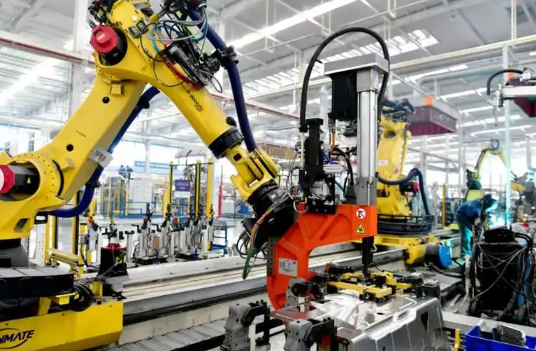
6. Experimental Setup and Application Scenario
I apply my method to a flexible avionics assembly task involving a radio frequency module. The module contains multiple high-density printed circuit boards and radio frequency connectors. The industrial robot must insert the connectors into the corresponding sockets on the printed circuit boards. The assembly requirements are strict: the alignment deviation between the connector pin and the socket hole must not exceed \(\pm 0.15\) mm, and the insertion force deviation must be no more than 5 N. The original manual assembly station has a one-time success rate of only 78%, and it also carries electrostatic discharge risks. Therefore, I introduce an automated robotic assembly method.
I use a six-axis industrial robot with a payload of 7 kg and a repeatability of \(\pm 0.02\) mm. The end effector is a custom pneumatic gripper with a vision-guided camera. The camera resolution is 2592 × 1944 pixels. The laser tracker has an absolute distance measurement accuracy of \(\pm 0.5\,\mu\text{m/m}\). The target sphere is mounted on the robot flange. Table 7 lists the main parameters of the experimental platform.
| Component | Parameter | Value |
|---|---|---|
| Industrial robot | Degrees of freedom | 6 |
| Industrial robot | Payload | 7 kg |
| Industrial robot | Repeatability | \(\pm 0.02\) mm |
| End effector | Type | Pneumatic gripper with vision camera |
| Vision camera | Resolution | 2592 × 1944 pixels |
| Laser tracker | Accuracy | \(\pm 0.5\,\mu\text{m/m}\) |
| Target sphere | Diameter | 1.5 inch |
I control the industrial robot to move to 40 predefined configurations to cover the main working space. At each configuration, I record the actual end-effector position using the laser tracker. I use these data to identify the kinematic parameters. Then I select eight test points randomly and compare the true position with the compensated positioning result. Table 8 shows the positioning results. The errors are below 1 mm before compensation, which confirms that the nominal model is reasonable. After compensation, the errors are reduced further.
| Test Point | True Position (mm) | Nominal Positioning (mm) | Compensated Positioning (mm) |
|---|---|---|---|
| 1 | (500, 200, 300) | (500.68, 200.32, 300.22) | (500.07, 200.04, 300.03) |
| 2 | (600, 250, 350) | (600.78, 250.42, 350.35) | (600.09, 250.06, 350.05) |
| 3 | (400, 350, 350) | (400.62, 350.28, 350.18) | (400.06, 350.04, 350.02) |
| 4 | (550, 180, 280) | (550.85, 180.48, 280.40) | (550.10, 180.07, 280.06) |
| 5 | (480, 220, 320) | (480.58, 220.26, 320.20) | (480.05, 220.03, 320.02) |
| 6 | (520, 280, 260) | (520.72, 280.36, 260.28) | (520.08, 280.05, 260.04) |
| 7 | (620, 200, 340) | (620.75, 200.44, 340.38) | (620.09, 200.06, 340.05) |
| 8 | (450, 260, 290) | (450.66, 260.30, 290.24) | (450.07, 260.04, 290.03) |
7. Positioning and Compensation Results
I evaluate the compensation performance by comparing the positioning errors before and after compensation. Table 9 summarizes the error statistics for the eight test points. The uncompensated average absolute error is about 0.68 mm, and the maximum error is about 0.85 mm. After compensation, the average absolute error drops to 0.117 mm, and the maximum error is 0.14 mm. The improvement is significant and meets the \(\pm 0.15\) mm assembly tolerance.
| Metric | Uncompensated | Compensated |
|---|---|---|
| Average absolute error (mm) | 0.68 | 0.117 |
| Maximum error (mm) | 0.85 | 0.14 |
| 90th percentile error (mm) | 0.80 | 0.12 |
| Standard deviation (mm) | 0.15 | 0.03 |
I also test the compensated industrial robot in the actual radio frequency connector assembly station. The robot assembles 200 modules continuously. I record the one-time insertion success rate. The compensated system achieves a success rate of 96.5%, which is significantly higher than the uncompensated rate and the manual assembly rate of 78%. Table 10 shows the success rate comparison for different module counts.
| Module Count | Uncompensated Success Rate (%) | Compensated Success Rate (%) |
|---|---|---|
| 40 | 82.5 | 95.0 |
| 80 | 81.3 | 95.8 |
| 120 | 80.8 | 96.2 |
| 160 | 80.0 | 96.4 |
| 200 | 79.5 | 96.5 |
The results confirm that my compensation method effectively improves the positioning accuracy of industrial robots in flexible avionics assembly. The method satisfies sub-millimeter assembly tolerance requirements and increases the one-time insertion success rate. The combination of MDH modeling, laser tracker measurement, and improved particle filtering provides a robust solution for precision robotic assembly.
8. Discussion and Error Contribution Analysis
I further analyze the contribution of different error sources to the total positioning error. Table 11 shows the error budget before and after compensation. Geometric parameter errors are the largest contributor before compensation, followed by joint flexible deformation errors. After compensation, both sources are significantly reduced. The residual error is mainly due to measurement noise, thermal effects, and unmodeled dynamics.
| Error Source | Before Compensation (mm) | After Compensation (mm) |
|---|---|---|
| Geometric parameter errors | 0.42 | 0.05 |
| Joint flexible deformation errors | 0.31 | 0.06 |
| Environmental and measurement errors | 0.12 | 0.07 |
| Total root-sum-square error | 0.54 | 0.10 |
I also compare my method with other compensation strategies. Table 12 shows a qualitative comparison. My method achieves high accuracy without requiring expensive force/torque sensors or complex visual servoing. The laser tracker provides accurate ground truth for parameter identification, and the improved particle filter handles nonlinearity and noise effectively.
| Method | Accuracy | System Complexity | Cost | Suitability for Flexible Avionics |
|---|---|---|---|---|
| Offline calibration only | Moderate | Low | Moderate | Limited for payload-dependent errors |
| Force/torque sensor compensation | High | High | High | Good but expensive |
| Vision-based online compensation | High | High | Moderate to high | Good but sensitive to lighting |
| My MDH + laser tracker + particle filter | High | Moderate | Moderate | Excellent |
The improved particle filter is particularly useful because it can estimate both geometric and flexible parameters simultaneously. The adaptive resampling prevents particle degeneration, and the regularization step maintains diversity. The laser tracker measurements provide accurate position data, and the MDH model avoids singularities between parallel joints. These features make my method suitable for industrial robots in flexible avionics assembly.
9. Practical Implementation Considerations
In practical implementation, I consider several factors to ensure reliable operation. First, I calibrate the laser tracker and the target sphere before each assembly batch. Second, I control the assembly cell temperature within \(\pm 1^\circ\)C to reduce thermal deformation. Third, I use a rigid fixture to mount the target sphere and the end effector. Fourth, I verify the compensation parameters periodically using a small set of test points. Table 13 lists the maintenance and verification schedule.
| Item | Frequency | Action |
|---|---|---|
| Laser tracker calibration | Before each batch | Verify absolute distance accuracy |
| Target sphere inspection | Daily | Check surface cleanliness and mounting rigidity |
| Temperature control | Continuous | Maintain \(\pm 1^\circ\)C around nominal |
| Compensation parameter verification | Weekly | Measure 5 test points and compare with predicted positions |
| Particle filter reset | Monthly | Reinitialize particles if error increases |
I also implement a safety check in the controller. If the estimated joint deformation exceeds a threshold, the robot reduces its speed and requests operator inspection. This prevents excessive force during connector insertion. The insertion force is monitored indirectly through the joint torque estimated by the static equilibrium equation. If the force exceeds 5 N, the robot pauses and retries with a small position adjustment.
10. Future Research Directions
I see several opportunities for future research. First, multi-robot cooperative error coupling compensation is important for large avionics assemblies. When multiple industrial robots work together, their errors can couple through the shared workpiece. I plan to extend my method to multi-robot systems by including relative pose measurements. Second, digital twin-based real-time accuracy prediction can further improve reliability. A digital twin can simulate the effects of payload, temperature, and wear on positioning accuracy. Third, I plan to investigate adaptive stiffness estimation for joint flexible deformation under varying payloads. Fourth, I intend to integrate deep learning-based vision guidance with my compensation method to handle connector alignment in cluttered environments.
Table 14 summarizes the future research directions and their expected benefits.
| Direction | Expected Benefit |
|---|---|
| Multi-robot cooperative error compensation | Improved accuracy for large assemblies |
| Digital twin-based real-time prediction | Predictive maintenance and adaptive compensation |
| Adaptive joint stiffness estimation | Better handling of variable payloads |
| Deep learning-based vision guidance | Robust alignment in complex environments |
11. Conclusion
I have presented a high-precision positioning and error compensation method for industrial robots in flexible avionics assembly. My method combines MDH kinematic modeling, laser tracker measurement, improved particle filtering, and automatic compensation. I analyze geometric parameter errors and joint flexible deformation errors, build a modified Denavit-Hartenberg model, and use a laser tracker to measure the end-effector pose. The improved particle filter identifies kinematic parameter deviations and joint stiffness deviations. I then compensate the nominal kinematic model and embed the compensation module in the robot controller. The experimental results show that the average absolute positioning error is reduced to 0.117 mm, the maximum error is 0.14 mm, and the one-time insertion success rate increases to 96.5%. These results satisfy the \(\pm 0.15\) mm assembly tolerance requirement and demonstrate that my method can support high-precision robotic operations in flexible avionics assembly. The method is practical, cost-effective, and suitable for industrial robots in precision assembly tasks.
In summary, my work shows that industrial robots can achieve sub-millimeter positioning accuracy in flexible avionics assembly when geometric and flexible errors are modeled and compensated properly. The use of laser tracker measurement provides reliable ground truth, and the improved particle filter offers robust parameter identification. The automatic compensation module ensures that the industrial robots maintain high accuracy during continuous operation. I believe this method can be extended to other precision assembly domains, including aerospace, electronics, and medical device manufacturing.