
The rotary vector reducer represents an emerging transmission technology developed from traditional cycloidal-pin wheel planetary drives. It overcomes the shortcomings of standard cycloidal drives while offering a series of advantages such as compact size, light weight, a wide range of transmission ratios, long service life, stable precision retention, high efficiency, and smooth operation. Consequently, it has garnered extensive attention globally. Due to its numerous benefits, including high torque capacity, strong impact resistance, high positioning accuracy, low vibration, and a large reduction ratio, the rotary vector reducer is widely used in industrial robots, machine tools, medical detection equipment, and satellite reception systems. Currently, high-precision robots in many countries utilize rotary vector reducers for transmission, making this technology a focal point in academic research and technological development.
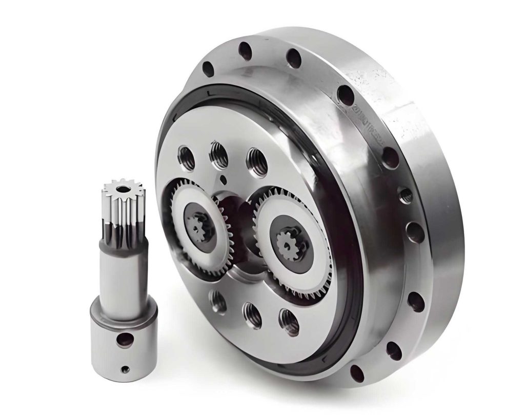
The core mechanism of a rotary vector reducer, often referred to as an RV reducer, typically consists of a two-stage, crank-enclosed differential gear train. The first stage is an involute planetary gear train, and the second stage is a cycloidal-pin wheel transmission. This is not a simple series connection but a functionally integrated system. The primary components include a gear shaft (input), planetary gears, crank shafts, cycloidal discs, a pin wheel (or ring gear with pins), a pin housing, and a planet carrier (output).
In operation, the motor drives the central gear shaft. The planetary gears, meshing with the central gear, rotate on their own axes while revolving around the central gear axis, completing the first stage of speed reduction. The crank shafts are fixed to the planetary gears, inheriting their compound motion. These crank shafts, via eccentric bearings, drive two cycloidal discs in an eccentric motion. The cycloidal discs mesh with the stationary pin ring. Due to the unique profile of the cycloidal teeth and the constraint of the pins, the cycloidal discs undergo a planetary motion: they revolve around the central axis of the pin ring while simultaneously rotating on their own axes. This rotation is transmitted through the crank shafts to the planet carrier, which acts as the output, achieving the second, more significant stage of speed reduction.
Within this sophisticated system of the rotary vector reducer, angular contact ball bearings play a critical role. These are often thin-section bearings serving as the main support bearings for the entire unit. They withstand combined loads including bending moments and torques. Their ability to carry both radial and axial loads makes the analysis of their loading conditions essential for reliable design and operation.
Load Capacity Calculation for Angular Contact Ball Bearings
Consider an angular contact ball bearing, such as type 76182B, with a contact angle $\alpha = 40^\circ$ and $Z = 51$ balls. The bearing’s position and the loading from the rotary vector reducer are defined by several key parameters.
| Parameter | Symbol | Value |
|---|---|---|
| Distance from Bearing 1 to input point | $a$ | 165.23 mm |
| Distance from Bearing 2 to input point | $b$ | 40.83 mm |
| Input (sun) gear radius | $r_1$ | 14.875 mm |
| Planetary gear radius (pitch circle) | $r_2$ | 98 mm |
| Instantaneous maximum input torque | $T_{max_i}$ | 20.24 Nm |
| Instantaneous maximum allowable bending moment | $M_c$ | 4900 Nm |
| Maximum allowable thrust (axial) load | $F_A$ | 13.72 kN |
| Gear pressure angle | $\alpha_g$ | $20^\circ$ |
1. Calculation of Radial Loads on the Bearings
The tangential force from the input torque is:
$$F_T = \frac{T_{max_i}}{r_1} = \frac{20.24}{0.014875} \approx 1360.54 \text{ N}$$
The corresponding separating radial force from the gear mesh is:
$$F_R = F_T \cdot \tan(\alpha_g) = 1360.54 \cdot \tan(20^\circ) \approx 495.2 \text{ N}$$
Considering force and moment equilibrium in the plane containing the radial gear force (XOY plane) and the plane containing the tangential gear force (XOZ plane), the radial reaction forces $F_{Rr1}$ and $F_{Rr2}$ from the bearings due to $F_R$ and $M_c$, and $F_{Tr1}$ and $F_{Tr2}$ due to $F_T$, can be solved. The governing equations are:
For XOY plane (Radial gear force $F_R$ and moment $M_c$):
$$ \frac{F_{Rr1} + F_{Rr2}}{2} = F_R $$
$$ (a+b)F_{Rr1} – a F_R = M_c $$
For XOZ plane (Tangential gear force $F_T$):
$$ F_{Tr1} + F_{Tr2} = F_T $$
$$ (a+b)F_{Tr1} = b F_T $$
The total radial load on each bearing is the vector sum of its components:
$$ F_{r1} = \sqrt{F_{Rr1}^2 + F_{Tr1}^2} $$
$$ F_{r2} = \sqrt{F_{Rr2}^2 + F_{Tr2}^2} $$
Solving these equations yields:
$$ F_{r1} \approx 17.35 \text{ kN}, \quad F_{r2} \approx 17.88 \text{ kN} $$
2. Calculation of Axial Loads on the Bearings
For an angular contact ball bearing with $\alpha = 40^\circ$, the induced or derived axial force is approximately $F_d = 1.14 F_r$.
Therefore:
$$ F_{d1} = 1.14 \times F_{r1} \approx 19.78 \text{ kN} $$
$$ F_{d2} = 1.14 \times F_{r2} \approx 20.38 \text{ kN} $$
To find the actual axial loads $F_{a1}$ and $F_{a2}$, we consider the external axial load $F_A$ and the equilibrium. The rule is: the bearing with the larger resultant axial load on its raceway is the one that carries the net external thrust.
Since $F_A + F_{d1} = 13.72 + 19.78 = 33.5 \text{ kN} > F_{d2} = 20.38 \text{ kN}$, Bearing 1 is “relaxed” and Bearing 2 is “loaded”.
Thus:
$$ F_{a1} = F_{d1} = 19.78 \text{ kN} $$
$$ F_{a2} = F_A + F_{d1} = 33.5 \text{ kN} $$
Internal Load Distribution in the Angular Contact Ball Bearing
The next step is to determine how the calculated radial and axial loads distribute among the rolling elements. This is governed by the relative load parameter $e$ and the load distribution integrals $J_r(\epsilon)$. For the bearings in the rotary vector reducer, we evaluate the ratio $F_a / (F_r \cdot \tan\alpha)$.
For Bearing 1: $$ \frac{F_{a1}}{F_{r1} \cdot \tan(40^\circ)} \approx 1.265 $$
For Bearing 2: $$ \frac{F_{a2}}{F_{r2} \cdot \tan(40^\circ)} \approx 2.235 $$
Using standard load distribution tables or calculations, we find the load distribution factor $\epsilon$ and the radial integral $J_r(\epsilon)$ for each case.
- Bearing 1: $\epsilon_1 \approx 0.7155$, leading to a load zone less than $180^\circ$.
- Bearing 2: $\epsilon_2 \approx 1.2288$, indicating a load zone greater than $180^\circ$ (over half the bearing is loaded).
The maximum normal contact load on any ball, $Q_{max}$, is given by:
$$ Q_{max} = \frac{F_r}{Z \cdot J_r(\epsilon) \cdot \cos\alpha} $$
Thus:
$$ Q_{max1} = \frac{17350}{51 \cdot J_r(0.7155) \cdot \cos(40^\circ)} \approx 1766.92 \text{ N} $$
$$ Q_{max2} = \frac{17880}{51 \cdot J_r(1.2288) \cdot \cos(40^\circ)} \approx 1980.53 \text{ N} $$
The load at any angular position $\phi_i$ relative to the load line is:
$$ Q(\phi_i) = Q_{max} \left[ 1 – \frac{1}{2\epsilon}(1 – \cos\phi_i) \right]^{1.5} \quad \text{for} \quad |\phi_i| \leq \phi_{load\ zone} $$
The calculated loads for each ball position are summarized below.
| Angular Position $\phi_i$ (°) | Contact Load $Q_1(\phi)$ (N) – Bearing 1 | Contact Load $Q_2(\phi)$ (N) – Bearing 2 |
|---|---|---|
| 0 | 1766.92 | 1980.53 |
| 7.06 | 1752.90 | 1971.37 |
| 14.12 | 1711.28 | 1944.13 |
| 21.18 | 1643.34 | 1899.46 |
| 28.24 | 1551.19 | 1838.45 |
| 35.29 | 1437.67 | 1762.55 |
| 42.35 | 1306.30 | 1673.57 |
| 49.41 | 1161.10 | 1573.58 |
| 56.47 | 1006.54 | 1464.87 |
| 63.53 | 847.35 | 1349.86 |
| 70.59 | 688.42 | 1231.06 |
| 77.65 | 534.61 | 1110.94 |
| 84.71 | 390.71 | 991.88 |
| 91.76 | 261.33 | 876.12 |
| 98.82 | 150.98 | 765.66 |
| 105.88 | 64.42 | 662.23 |
| 112.94 | 8.64 | 567.23 |
| 120.00 | 0.00 | 481.72 |
| 127.06 | 0.00 | 406.39 |
| 134.12 | 0.00 | 341.58 |
| 141.18 | 0.00 | 287.32 |
| 148.23 | 0.00 | 243.34 |
| 155.29 | 0.00 | 209.19 |
| 162.35 | 0.00 | 184.30 |
| 169.41 | 0.00 | 168.09 |
| 176.47 | 0.00 | 160.12 |
3. Hertzian Contact Stress and Deformation
Applying Hertzian contact theory to the point of maximum load ($Q_{max}$) between the ball and the outer raceway allows us to calculate the contact ellipse dimensions, the maximum contact stress, and the elastic approach. The calculations require the geometric and material properties (equivalent radii of curvature, $\Sigma\rho$, and elastic moduli).
The semi-major axis $a$ and semi-minor axis $b$ of the contact ellipse are:
$$ a = a^* \left( \frac{Q}{\Sigma\rho} \right)^{1/3}, \quad b = b^* \left( \frac{Q}{\Sigma\rho} \right)^{1/3} $$
where $a^*$ and $b^*$ are dimensionless coefficients dependent on the curvature difference.
The maximum contact stress $\sigma_{max}$ at the center of the ellipse is:
$$ \sigma_{max} = \frac{3Q}{2\pi a b} $$
The mutual approach (deformation) $\delta$ between the ball and raceway is:
$$ \delta = \delta^* \left( \frac{Q^2}{\Sigma\rho} \right)^{1/3} $$
where $\delta^*$ is a corresponding deformation coefficient.
The following table summarizes the key Hertzian coefficients and the calculated results for the outer raceway contact in the rotary vector reducer bearings.
| Parameter | Bearing 1 | Bearing 2 |
|---|---|---|
| Ellipse Semi-major Axis Coefficient, $a^*$ | 3.1811 | 3.1811 |
| Ellipse Semi-minor Axis Coefficient, $b^*$ | 0.4543 | 0.4543 |
| Deformation Coefficient, $\delta^*$ | 0.67 | 0.67 |
| Semi-major Axis, $a$ (mm) | 1.5635 | 1.6241 |
| Semi-minor Axis, $b$ (mm) | 0.2233 | 0.2319 |
| Max Contact Stress, $\sigma_{max}$ (MPa) | 2416.52 | 2510.22 |
| Max Contact Deformation, $\delta_{max}$ (mm) | 0.0159 | 0.0171 |
Finite Element Simulation and Verification
To validate the analytical load calculations for the angular contact ball bearing within the rotary vector reducer assembly, a finite element analysis (FEA) was conducted. Given the large size and thin-section nature of the bearing (76182B), a full-model simulation with all 51 balls would be computationally prohibitive. Since the performance is critically influenced by the most heavily loaded rolling element, the analysis focused on a simplified sub-model containing a single ball in contact with the inner and outer raceway segments.
The boundary conditions were set to reflect the operating state in the rotary vector reducer: the outer raceway was fixed, while the inner raceway was subjected to the combined radial and axial loads calculated earlier ($F_{r1}$, $F_{a1}$ for Bearing 1 and $F_{r2}$, $F_{a2}$ for Bearing 2). Advanced nonlinear surface-to-surface contact was defined with appropriate normal and tangential penalty factors. A static structural analysis was performed to solve for the contact forces and stresses.
The simulation results for contact force and maximum contact stress on the most loaded ball were extracted. The comparison between the theoretical Hertzian calculations and the FEA results is presented below.
| Metric | Bearing 1 | Bearing 2 | ||
|---|---|---|---|---|
| Theory | FEA | Theory | FEA | |
| Contact Force, $Q_{max}$ (N) | 1766.92 | 1757.82 | 1980.53 | 1990.20 |
| Max Contact Stress, $\sigma_{max}$ (MPa) | 2416.52 | 2362.89 | 2510.22 | 2527.42 |
| Relative Error | – | ~0.5% (Force) ~2.2% (Stress) |
– | ~0.5% (Force) ~0.7% (Stress) |
The close agreement between the analytical and simulation results validates both the load distribution calculations for the bearing and the FEA modeling parameters. The minor discrepancies arise from the approximations inherent in the analytical load integral methods and the specific contact algorithm settings (friction, penalty factors, convergence criteria) in the FEA. This confirms that the simplified analytical approach, considering the high rigidity and precision of the rotary vector reducer system and the preload condition of the bearings, accurately reflects the operational state of the angular contact ball bearings.
Conclusion
This analysis comprehensively examined the load distribution and contact mechanics of angular contact ball bearings within a rotary vector reducer. Starting from the operating principle and load transmission path of the RV reducer, the radial and axial loads on the main support bearings were calculated using static equilibrium. Subsequently, the internal load distribution among the rolling elements and the resulting maximum Hertzian contact stress and deformation were determined analytically. Finally, a finite element simulation of a critical bearing section was performed, yielding results that strongly corroborated the theoretical calculations.
The maximum calculated contact stress (approximately 2510 MPa) for the bearing under the specified extreme rotary vector reducer operating conditions is well below the allowable limit for high-quality bearing steel (often cited as 4200 MPa). In fact, experience suggests that ball bearings with contact stresses below 1500 MPa can be considered to have infinite fatigue life. The stresses found here, while higher than this conservative threshold, confirm the geometric parameter design’s adequacy for the demanding application within the rotary vector reducer.
This integrated analytical and simulation methodology provides a solid foundation for understanding the performance of angular contact ball bearings in rotary vector reducers. It offers a reliable and efficient tool for verifying bearing selection and load capacity during the design phase of a rotary vector reducer system, ensuring both reliability and longevity.