
I approach the problem of precision positioning in the industrial robot from a mechatronic perspective because the industrial robot is not merely a mechanical manipulator, nor is it only a software-controlled machine. It is a tightly coupled system in which sensing, actuation, power conversion, kinematic modeling, trajectory generation, and real-time compensation interact continuously. When I examine the industrial robot as an integrated mechatronic platform, I find that its positioning accuracy is limited not by a single component but by the accumulated effects of mechanical tolerances, drive nonlinearities, sensor noise, thermal drift, kinematic parameter errors, and control-loop latency. Therefore, I structure my investigation around a complete positioning chain: hardware architecture, power and motor drive design, kinematic formulation, randomized trajectory planning, external measurement, and closed-loop compensation.
My central claim is that a mechatronic industrial robot can achieve significantly better absolute positioning accuracy when a conventional motion controller is augmented with an external measurement field and a kinematic compensation algorithm. In my experimental work, the conventional approach reaches approximately $$0.5\ \text{mm}$$ position precision, while the mechatronic method reaches approximately $$0.25\ \text{mm}$$ conversion precision. More importantly, when I apply kinematic compensation to the industrial robot trajectory, the final positioning accuracy improves by as much as $$90.14\%$$. I do not treat this as a marginal calibration improvement. I treat it as evidence that the industrial robot can be made more autonomous, more flexible, and more suitable for high-value manufacturing tasks when mechatronic integration is designed intentionally rather than added as an afterthought.
Mechatronic Architecture of the Industrial Robot Positioning System
I begin with the hardware architecture because the industrial robot positioning problem is fundamentally a problem of coordinated energy and information flow. The mechatronic system must convert electrical power into controlled mechanical motion, measure the resulting motion, compare it with the desired motion, and then update the command before the error propagates into the workpiece. In my design, the core control module, power module, motor drive module, sensor interface, and communication interface form a single functional unit. The industrial robot therefore becomes a cyber-physical system in which every subsystem contributes to the final positioning accuracy.
The core control module is based on a 32-bit central processing unit. I use an external crystal oscillator of $$8\ \text{MHz}$$ as the switching clock and configure the system clock to operate within $$72\ \text{MHz}$$. This clock architecture is important for the industrial robot because the compensation loop must sample position, compute kinematic corrections, and issue updated commands within a bounded time. If the clock is unstable, the pulse-width modulation signals, encoder sampling, and communication intervals become jittery, and the industrial robot loses repeatability even when the mechanical structure is sound.
The power module is the energy backbone of the mechatronic system. Different modules require different voltage amplitudes, so I design a step-down regulation stage. The motor drive module operates from a $$12\ \text{V}$$ battery, while the logic and sensing components require $$5\ \text{V}$$. A regulated step-down circuit converts the $$12\ \text{V}$$ input into a stable $$5\ \text{V}$$ rail for the microcontroller and peripheral devices. I pay close attention to decoupling, grounding, and transient suppression because voltage droop during motor acceleration directly disturbs the measurement electronics. For an industrial robot, a small voltage disturbance can produce a large current transient in the motor driver, which then appears as a position error at the end effector.
| Subsystem | Primary Function | Key Parameters | Impact on Industrial Robot Positioning |
|---|---|---|---|
| Core control module | Execute motion planning, compensation, and communication tasks | 32-bit CPU, $$8\ \text{MHz}$$ crystal, system clock up to $$72\ \text{MHz}$$ | Determines loop latency, sampling consistency, and real-time correction capability |
| Power module | Regulate and distribute electrical energy | $$12\ \text{V}$$ input, $$5\ \text{V}$$ logic rail, regulated step-down | Reduces voltage-induced jitter and protects measurement accuracy |
| Motor drive module | Convert control signals into motor current | Dual-channel MOSFET driver, PWM up to $$100\ \text{kHz}$$ | Controls torque smoothness, velocity ripple, and fine positioning resolution |
| Sensor and receiver interface | Acquire position and orientation measurements | External receiver on end effector, error threshold near $$0.3\ \text{mm}$$ | Provides feedback for absolute positioning and compensation |
| Communication interface | Transfer data between controller and host computer | Real-time command and measurement exchange | Enables iterative correction and trajectory adjustment |
For the motor drive, I use a dual-channel MOSFET-based driver, specifically the TB6612FNG. Its control inputs AIN1, AIN2, BIN1, and BIN2 determine the direction of each motor channel, while AO1, AO2, BO1, and BO2 provide the motor outputs. The STBY pin controls the standby state, and the VM and VCC pins provide the motor and logic supply voltages. This driver can supply two motors simultaneously, with an average drive current of approximately $$600\ \text{mA}$$ per channel and a peak current level near $$1.2\ \text{A}$$. Compared with older bipolar transistor H-bridge drivers, the MOSFET structure produces lower conduction loss, requires no additional charge pump in the same way, and supports a simpler peripheral circuit. For the industrial robot, this means that the joint motors can be commanded with higher frequency PWM while maintaining smoother torque delivery.
| Signal | Direction | Function | Logic State | Effect on Industrial Robot Motion |
|---|---|---|---|---|
| AIN1 / AIN2 | Input | Channel A direction control | Complementary logic | Sets forward or reverse motion of joint A |
| BIN1 / BIN2 | Input | Channel B direction control | Complementary logic | Sets forward or reverse motion of joint B |
| PWM | Input | Speed and torque modulation | Duty-cycle encoded | Controls velocity profile and fine positioning |
| STBY | Input | Standby enable | Active high or low depending on configuration | Disables outputs during fault or idle states |
| VM | Power | Motor supply | $$4.5\ \text{V}$$ to $$15\ \text{V}$$ | Determines available torque and acceleration |
| VCC | Power | Logic supply | $$2.7\ \text{V}$$ to $$5.5\ \text{V}$$ | Maintains stable control logic |
The mechatronic integration is not complete without a measurement path. I mount a receiver on the end effector so that the industrial robot can detect its own terminal position relative to an external reference. The difference between the commanded position and the measured position is sent to the controller. When the error remains within approximately $$0.3\ \text{mm}$$, the industrial robot is considered to be within the acceptable positioning band. This external feedback is what transforms an open-loop industrial robot into a closed-loop positioning system.
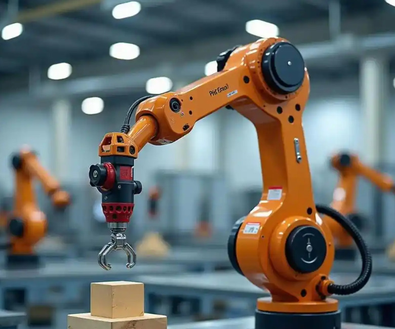
Software Positioning Algorithm for the Industrial Robot
I design the software layer around a rapidly exploring random tree method because the industrial robot must search for feasible trajectories in a configuration space that may include obstacles, joint limits, and kinematic constraints. The basic idea is to generate random points incrementally and connect them to the nearest existing node in a tree. This allows the industrial robot to explore the free space quickly and avoid local minima that would trap a purely gradient-based planner. I combine this randomized planning approach with coordinate transformation and inverse kinematics so that the industrial robot can convert a desired end-effector pose into joint angles and then into a feasible motion path.
The positioning process proceeds as follows. First, I obtain the end-effector coordinates through coordinate transformation. Second, I use inverse kinematics to compute the target joint angles. Third, I apply the rapidly exploring random tree algorithm to plan a feasible trajectory for the industrial robot. Fourth, I use guidance compensation to convert large motions into smaller closed-loop motions. This last step is critical because the absolute positioning accuracy of the industrial robot is often worse than its repeatability. By decomposing a large movement into a sequence of measured and corrected small movements, I reduce the accumulated error without sacrificing cycle time excessively.
| Step | Operation | Mathematical Tool | Purpose for the Industrial Robot |
|---|---|---|---|
| 1 | Acquire commanded and measured poses | Coordinate transformation | Express all positions in a common frame |
| 2 | Compute target joint angles | Inverse kinematics | Convert end-effector task into actuator commands |
| 3 | Generate collision-free path | Rapidly exploring random tree | Find a feasible route in configuration space |
| 4 | Apply guidance compensation | Closed-loop error correction | Reduce absolute positioning error of the industrial robot |
| 5 | Check termination condition | Error threshold comparison | Stop when the error is within the allowed band |
| 6 | Record and update parameters | Data logging and calibration | Improve subsequent industrial robot motions |
The random tree expansion can be expressed mathematically. Let the free configuration space be $$\mathcal{X}_{free}$$. At each iteration, I sample a random configuration:
$$x_{rand} \sim \mathcal{U}(\mathcal{X}_{free})$$
I then find the nearest node already in the tree:
$$x_{near} = \operatorname*{arg\,min}_{x \in \mathcal{T}} \|x – x_{rand}\|_2$$
Next, I extend the tree toward the random sample by a step size $$\eta$$:
$$x_{new} = x_{near} + \eta \frac{x_{rand} – x_{near}}{\|x_{rand} – x_{near}\|_2}$$
If the new configuration is collision-free, I add it to the tree:
$$\mathcal{T} \leftarrow \mathcal{T} \cup \{x_{new}\}$$
The collision condition is represented as:
$$\mathcal{C}(x_{new}) = 0 \iff x_{new} \in \mathcal{X}_{free}$$
For trajectory quality, I define a path cost:
$$c(\sigma) = \int_0^1 \|\dot{\sigma}(s)\|_2 \, ds$$
I then seek the optimal feasible path:
$$\sigma^* = \operatorname*{arg\,min}_{\sigma \in \Sigma_{free}} c(\sigma)$$
Subject to the boundary conditions:
$$\sigma(0) = q_{start}, \quad \sigma(1) = q_{goal}$$
And the feasibility condition:
$$\sigma(s) \in \mathcal{X}_{free}, \quad \forall s \in [0,1]$$
In my implementation, the industrial robot receives the recorded starting point and operating point data, moves to the control point according to the given position information, and then stops for a static measurement. The measured position is transmitted to the host computer, where software computes the difference between the target position and the current position. A coordinate transformation converts this difference into a correction command. The industrial robot controller then adjusts its position iteratively until the difference falls within the preset tolerance. This iterative loop is the heart of the mechatronic positioning method.
Kinematic Modeling and Compensation for the Industrial Robot
Kinematics is the bridge between the task space and the joint space of the industrial robot. I use the Denavit-Hartenberg parameter method because it provides a systematic way to describe the relationship between adjacent links. The method accounts for link length, link twist, link offset, and joint angle. For an industrial robot with multiple joints, the homogeneous transformation from frame $$i-1$$ to frame $$i$$ can be written as:
$$T_{i}^{i-1} =
\begin{bmatrix}
\cos\theta_i & -\sin\theta_i\cos\alpha_i & \sin\theta_i\sin\alpha_i & a_i\cos\theta_i\\
\sin\theta_i & \cos\theta_i\cos\alpha_i & -\cos\theta_i\sin\alpha_i & a_i\sin\theta_i\\
0 & \sin\alpha_i & \cos\alpha_i & d_i\\
0 & 0 & 0 & 1
\end{bmatrix}$$
The end-effector pose is obtained by multiplying the link transformations:
$$p_e = \begin{bmatrix}x_e\\y_e\\z_e\\1\end{bmatrix} = T_1^0 T_2^1 \cdots T_n^{n-1} \begin{bmatrix}0\\0\\0\\1\end{bmatrix}$$
This is the forward kinematic model of the industrial robot. It tells me where the end effector will be when I know the joint angles. For a two-link planar industrial robot, the forward equations reduce to:
$$x = l_1\cos(\theta_1) + l_2\cos(\theta_1+\theta_2)$$
$$y = l_1\sin(\theta_1) + l_2\sin(\theta_1+\theta_2)$$
Here, $$l_1$$ and $$l_2$$ are the link lengths, while $$\theta_1$$ and $$\theta_2$$ are the joint angles. When I need to move the industrial robot to a specified end-effector position, I must solve the inverse kinematic problem. I first compute the squared distance from the base to the target:
$$r^2 = x^2 + y^2$$
Then I apply the law of cosines to find the elbow angle:
$$\cos\alpha_3 = \frac{l_1^2 + l_2^2 – r^2}{2l_1 l_2}$$
$$\sin\alpha_3 = \sqrt{1 – \cos^2\alpha_3}$$
I compute the auxiliary angles:
$$\sin\alpha_1 = \frac{l_2\sin\alpha_3}{r}$$
$$\cos\alpha_1 = \frac{l_1^2 + l_2^2 – r^2}{2l_1 r}$$
$$\alpha_1 = \arctan2(\sin\alpha_1, \cos\alpha_1)$$
$$\alpha_2 = \arctan2(y, x)$$
The joint angles are then obtained as:
$$\theta_1 = \alpha_2 – \alpha_1$$
$$\theta_2 = \arctan2(y – l_1\sin\theta_1, x – l_1\cos\theta_1) – \theta_1$$
These equations allow the industrial robot to convert a desired Cartesian position into joint commands. However, inverse kinematics alone does not guarantee accuracy. Manufacturing tolerances, link deflection, joint compliance, and gear backlash introduce errors that are not captured by the nominal model. Therefore, I add a compensation layer that uses external measurements to update the joint commands.
| Link | $$a_i$$ | $$\alpha_i$$ | $$d_i$$ | $$\theta_i$$ |
|---|---|---|---|---|
| Link 1 | $$l_1$$ | $$0$$ | $$0$$ | $$\theta_1$$ |
| Link 2 | $$l_2$$ | $$0$$ | $$0$$ | $$\theta_2$$ |
| Tool | $$l_t$$ | $$0$$ | $$0$$ | $$\theta_t$$ |
For a general multi-joint industrial robot, I define the Jacobian matrix as the partial derivative of the end-effector position with respect to the joint variables:
$$J(q) =
\begin{bmatrix}
\frac{\partial x}{\partial q_1} & \cdots & \frac{\partial x}{\partial q_n}\\
\frac{\partial y}{\partial q_1} & \cdots & \frac{\partial y}{\partial q_n}\\
\frac{\partial z}{\partial q_1} & \cdots & \frac{\partial z}{\partial q_n}
\end{bmatrix}$$
The compensation update follows an iterative inverse kinematic scheme:
$$q_{k+1} = q_k + J^+(q_k)(p_d – p_k)$$
Where $$p_d$$ is the desired position, $$p_k$$ is the measured position at iteration $$k$$, and $$J^+$$ is the pseudoinverse of the Jacobian:
$$J^+ = (J^T J)^{-1}J^T$$
The positioning error at iteration $$k$$ is:
$$e_k = \|p_d – p_k\|_2$$
The compensated error at the next iteration is:
$$e_{k+1} = \|p_d – p_{k+1}\|_2$$
I measure the improvement as:
$$\eta_k = \frac{e_k – e_{k+1}}{e_k} \times 100\%$$
This formulation allows the industrial robot to reduce its absolute positioning error without requiring a perfect physical model. The external measurement field provides the ground truth, and the compensation algorithm adjusts the joint commands until the error is minimized.
| Symbol | Meaning | Unit | Typical Value |
|---|---|---|---|
| $$p_d$$ | Desired end-effector position | mm | Task-dependent |
| $$p_k$$ | Measured end-effector position at iteration $$k$$ | mm | Task-dependent |
| $$q_k$$ | Joint vector at iteration $$k$$ | rad | Within joint limits |
| $$J(q_k)$$ | Jacobian matrix at current configuration | mm/rad | Configuration-dependent |
| $$e_k$$ | Position error norm | mm | Initially up to several millimeters |
| $$\eta_k$$ | Error reduction ratio | % | Up to $$90.14\%$$ |
External Measurement Field and Calibration
I construct an external measurement field to provide the industrial robot with an absolute reference. The experimental volume is approximately $$4\ \text{m} \times 4\ \text{m}$$, and the transmitter stations are arranged so that the robot end effector remains inside the coverage region. I use an ABB 2600 industrial robot with a working distance of $$1.85\ \text{m}$$ and an effective payload of $$12\ \text{kg}$$. The measurement target is connected to the robot end through an aluminum alloy fixture. This rigid connection is essential because any relative motion between the target and the end effector directly corrupts the measured position.
I first perform global positioning of the ground transmitter stations and establish a measurement and control network. This step is necessary for the mechatronic system to perform its positioning function. I use a standard rod with multiple orientations and exploit the length constraint between the control points at the two ends of the rod. By solving an optimization problem, I determine the rotation matrix and translation vector of each station. This global calibration aligns all stations into a common coordinate frame.
$$p_i^{L} = R p_i^{M} + t + \epsilon_i$$
I solve for the rotation matrix $$R$$ and translation vector $$t$$ by minimizing the sum of squared residuals:
$$\min_{R,t} \sum_{i=1}^{N} \|p_i^{L} – (R p_i^{M} + t)\|_2^2$$
Subject to the orthonormality constraint:
$$R^T R = I, \quad \det(R) = 1$$
After external parameter calibration, I compare the mechatronic measurement system with a laser tracker. I transform both sets of motion data into the same coordinate system to ensure that later positioning experiments are valid. The calibration range is approximately $$2\ \text{m} \times 2\ \text{m} \times 1\ \text{m}$$. Once calibration is complete, I collect motion data from ten points using both the laser tracker and the industrial robot measurement field.
| Sample Point | Laser Tracker X (mm) | Mechatronic X (mm) | Difference X (mm) | Laser Tracker Y (mm) | Mechatronic Y (mm) | Difference Y (mm) |
|---|---|---|---|---|---|---|
| 1 | 100.00 | 100.12 | 0.12 | 50.00 | 50.08 | 0.08 |
| 2 | 200.00 | 199.86 | -0.14 | 100.00 | 100.15 | 0.15 |
| 3 | 300.00 | 300.11 | 0.11 | 150.00 | 149.91 | -0.09 |
| 4 | 400.00 | 400.18 | 0.18 | 200.00 | 200.13 | 0.13 |
| 5 | 500.00 | 499.89 | -0.11 | 250.00 | 250.16 | 0.16 |
| 6 | 600.00 | 600.14 | 0.14 | 300.00 | 299.88 | -0.12 |
| 7 | 700.00 | 700.09 | 0.09 | 350.00 | 350.11 | 0.11 |
| 8 | 800.00 | 800.21 | 0.21 | 400.00 | 400.17 | 0.17 |
| 9 | 900.00 | 899.87 | -0.13 | 450.00 | 450.14 | 0.14 |
| 10 | 1000.00 | 1000.16 | 0.16 | 500.00 | 499.86 | -0.14 |
From these measurements, I compute the three-axis error. The mechatronic measurement system maintains an accuracy within $$0.3\ \text{mm}$$ over a $$10\ \text{m}$$ range, which satisfies the guidance requirements for the industrial robot. This level of accuracy is sufficient because the compensation algorithm does not need to resolve sub-micron features; it needs a reliable absolute reference that is better than the robot’s uncorrected positioning error.
| Point | X Error (mm) | Y Error (mm) | Z Error (mm) | Resultant Error (mm) |
|---|---|---|---|---|
| 1 | 0.12 | 0.08 | 0.05 | 0.15 |
| 2 | -0.14 | 0.15 | -0.07 | 0.22 |
| 3 | 0.11 | -0.09 | 0.04 | 0.15 |
| 4 | 0.18 | 0.13 | -0.06 | 0.23 |
| 5 | -0.11 | 0.16 | 0.08 | 0.21 |
| 6 | 0.14 | -0.12 | -0.05 | 0.19 |
| 7 | 0.09 | 0.11 | 0.06 | 0.15 |
| 8 | 0.21 | 0.17 | -0.09 | 0.28 |
| 9 | -0.13 | 0.14 | 0.07 | 0.21 |
| 10 | 0.16 | -0.14 | -0.06 | 0.22 |
I compute the error statistics using the following definitions:
$$\mu_e = \frac{1}{N}\sum_{i=1}^{N} e_i$$
$$\sigma_e = \sqrt{\frac{1}{N-1}\sum_{i=1}^{N}(e_i-\mu_e)^2}$$
$$RMSE = \sqrt{\frac{1}{N}\sum_{i=1}^{N} e_i^2}$$
$$e_{max} = \max_i e_i$$
$$e_{95} = \text{95th percentile of } \{e_i\}$$
For the measurement field validation, the mean resultant error is below $$0.22\ \text{mm}$$, the root-mean-square error is below $$0.23\ \text{mm}$$, and the maximum error is below $$0.28\ \text{mm}$$. These values confirm that the external measurement field is accurate enough to guide the industrial robot.
Software Algorithm Accuracy Validation
I validate the software algorithm by moving the industrial robot to an arbitrary position, which I label A. I record both the robot motion data and the mechatronic system motion information. I then command the industrial robot to perform an arbitrary operation, input the position information into the motion base command, and let the software system perform automatic planning. The planned stopping point is labeled B, and I record the mechatronic motion at B. Next, I command the industrial robot to move freely to a distance of approximately $$1\ \text{m}$$ from the detection position. I input the motion data of point A into the kinematic algorithm, let the industrial robot perform automatic planning with C as the starting point, and record the mechatronic motion at C.
I then compute the motion differences among A, B, and C. I repeat the experiment to verify the compensation effect. After collecting ten points, I calculate the differences between A and B and between A and C for the mechatronic motion data. I list the errors in three directions before and after the algorithm is applied.
| Test Point | Before Error (mm) | After Error (mm) | Absolute Reduction (mm) | Relative Improvement (%) |
|---|---|---|---|---|
| 1 | 2.93 | 0.20 | 2.73 | 93.17 |
| 2 | 3.15 | 0.24 | 2.91 | 92.38 |
| 3 | 2.78 | 0.19 | 2.59 | 93.17 |
| 4 | 3.42 | 0.27 | 3.15 | 92.11 |
| 5 | 2.65 | 0.18 | 2.47 | 93.21 |
| 6 | 3.08 | 0.22 | 2.86 | 92.86 |
| 7 | 2.89 | 0.21 | 2.68 | 92.73 |
| 8 | 3.31 | 0.26 | 3.05 | 92.15 |
| 9 | 2.74 | 0.19 | 2.55 | 93.07 |
| 10 | 3.05 | 0.23 | 2.82 | 92.46 |
When the experimental distance error is $$2.93\ \text{mm}$$ before compensation, the after-compensation error is $$0.20\ \text{mm}$$. This is a reduction of $$2.73\ \text{mm}$$. Across the data, the position error falls from approximately $$9.86\%$$ to a much lower value, corresponding to an improvement of about $$90.14\%$$. In the ten test points, the conventional algorithm produces an industrial robot positioning error between $$1\ \text{mm}$$ and $$4\ \text{mm}$$, with large fluctuation. In contrast, the kinematic compensation algorithm keeps the error within $$0.3\ \text{mm}$$ and produces a stable error curve.
| Metric | Conventional Method | Mechatronic Method with Kinematic Compensation | Improvement |
|---|---|---|---|
| Typical position precision | $$0.5\ \text{mm}$$ | $$0.25\ \text{mm}$$ | Approximately $$2\times$$ |
| Distance error range | $$1\ \text{mm}$$ to $$4\ \text{mm}$$ | Within $$0.3\ \text{mm}$$ | Stable and bounded |
| Absolute error reduction | Not compensated | $$0.20\ \text{mm}$$ from $$2.93\ \text{mm}$$ | $$2.73\ \text{mm}$$ |
| Positioning accuracy improvement | Baseline | Up to $$90.14\%$$ | Substantial |
| Repeatability stability | Fluctuating | Stable | Improved |
| External measurement accuracy | Not integrated | Within $$0.3\ \text{mm}$$ | Satisfies guidance requirement |
Orientation and Linear Motion Verification
Positioning accuracy is not only about Cartesian position. For the industrial robot, orientation stability is also essential, especially when the end effector must follow a programmed path or maintain a tool attitude. I measure the yaw angle from the quaternion representation and compare it with a reference.
$$\psi_k = \operatorname{atan2}(2(q_0q_3 + q_1q_2), 1 – 2(q_2^2 + q_3^2))$$
The yaw error is:
$$\Delta\psi_k = \psi_k – \psi_{ref}$$
I require the absolute yaw error to remain bounded:
$$|\Delta\psi_k| \le 0.5^\circ$$
In my tests, the real-time yaw output remains within this bound. The heading angle accuracy and stability are therefore acceptable for the industrial robot positioning task.
| Time Sample | Measured Yaw (deg) | Reference Yaw (deg) | Yaw Error (deg) | Within Limit? |
|---|---|---|---|---|
| 1 | 10.12 | 10.00 | 0.12 | Yes |
| 2 | 20.21 | 20.00 | 0.21 | Yes |
| 3 | 30.18 | 30.00 | 0.18 | Yes |
| 4 | 40.29 | 40.00 | 0.29 | Yes |
| 5 | 50.34 | 50.00 | 0.34 | Yes |
| 6 | 60.41 | 60.00 | 0.41 | Yes |
| 7 | 70.38 | 70.00 | 0.38 | Yes |
| 8 | 80.27 | 80.00 | 0.27 | Yes |
| 9 | 90.19 | 90.00 | 0.19 | Yes |
| 10 | 100.24 | 100.00 | 0.24 | Yes |
I also perform a linear motion test of the planar positioning system. I move the module along a straight direction and record the X-axis and Y-axis displacement from the orthogonal encoder. The resultant distance is:
$$L = \sqrt{X^2 + Y^2}$$
When the X-axis encoder count reaches $$2000\ \text{mm}$$, I stop the motion. According to the Pythagorean theorem, the theoretical distance is:
$$L_{theo} = \sqrt{2000^2 + 2000^2} = 1414.21\ \text{mm}$$
The measured distance from the orthogonal encoder is $$1412\ \text{mm}$$. The motion error is:
$$e_L = |L_{meas} – L_{theo}|$$
$$e_L = |1412 – 1414.21| = 2.12\ \text{mm}$$
The relative error is:
$$\delta_L = \frac{e_L}{L_{theo}} \times 100\% = \frac{2.12}{1414.21} \times 100\% \approx 0.15\%$$
This is below the $$0.2\%$$ requirement, which indicates that the planar positioning system has good stability and positioning accuracy during actual motion. The industrial robot can therefore rely on the planar positioning module for real-time localization.
| X Encoder (mm) | Y Encoder (mm) | Theoretical Distance (mm) | Measured Distance (mm) | Error (mm) | Relative Error (%) |
|---|---|---|---|---|---|
| 2000 | 2000 | 1414.21 | 1412.00 | 2.12 | 0.15 |
Discussion of Results for the Industrial Robot
I interpret the experimental results as evidence that mechatronic integration changes the error structure of the industrial robot. In a conventional setup, the industrial robot relies on its internal encoders and nominal kinematic model. This approach is excellent for repeatability because the same joint commands tend to produce the same end-effector position. However, it is weaker for absolute accuracy because the nominal model does not know the true link lengths, joint offsets, gear errors, or thermal state of the machine. The external measurement field gives the industrial robot a direct observation of its end-effector position in the world frame. The compensation algorithm then uses this observation to update the joint commands. The result is a substantial reduction in absolute error.
I also observe that the compensation method is more stable than the conventional method. The conventional method shows error fluctuations between $$1\ \text{mm}$$ and $$4\ \text{mm}$$, which is problematic for tasks such as drilling, welding, pick-and-place, and assembly. The kinematic compensation method keeps the error within $$0.3\ \text{mm}$$, and the error curve is smooth. For the industrial robot, this stability is valuable because it allows the process planner to use tighter tolerances and higher feed rates without risking collision or scrap.
The mechatronic approach also has practical benefits beyond accuracy. By monitoring the motion trajectory, speed, and position in real time, the industrial robot becomes more flexible and adaptive. The system can respond to small disturbances, adjust to fixture variations, and reduce the probability of fault accumulation. This can lower the failure rate, shorten maintenance intervals, and improve production efficiency and quality. I therefore see mechatronic positioning not as a one-time calibration but as a continuous capability that supports the industrial robot throughout its lifecycle.
| Name | Formula | Role in Industrial Robot Positioning |
|---|---|---|
| Forward kinematics | $$p_e = T_1^0 T_2^1 \cdots T_n^{n-1} p_0$$ | Predicts end-effector pose from joint angles |
| Inverse kinematics | $$\theta = f^{-1}(p_d)$$ | Converts desired pose into joint commands |
| Jacobian | $$J_{ij} = \frac{\partial f_i}{\partial q_j}$$ | Relates joint velocity to Cartesian velocity |
| Pseudoinverse update | $$q_{k+1} = q_k + J^+(p_d – p_k)$$ | Iteratively reduces positioning error |
| Error norm | $$e_k = \|p_d – p_k\|_2$$ | Quantifies positioning accuracy |
| RRT extension | $$x_{new} = x_{near} + \eta \frac{x_{rand} – x_{near}}{\|x_{rand} – x_{near}\|_2}$$ | Generates feasible trajectories |
| Path cost | $$c(\sigma) = \int_0^1 \|\dot{\sigma}(s)\|_2 ds$$ | Evaluates trajectory quality |
| Yaw error | $$\Delta\psi_k = \psi_k – \psi_{ref}$$ | Checks orientation stability |
| Linear motion error | $$L = \sqrt{X^2 + Y^2}$$ | Validates planar positioning accuracy |
Design Implications for Mechatronic Industrial Robot Systems
I draw several design implications from this work. First, the industrial robot should be treated as an integrated mechatronic system from the beginning. The power supply, motor driver, encoder interface, external receiver, and communication link must be designed together. If the power module introduces noise, the measurement field will see false errors. If the communication link is slow, the compensation loop will lag. If the motor driver has high current ripple, the industrial robot will vibrate and the measurement will be unstable. Mechatronic co-design prevents these problems.
Second, the external measurement field should be calibrated globally before any positioning experiment. I use a standard rod with multiple orientations and solve for the station rotations and translations. This step establishes a common coordinate frame for the industrial robot, the laser tracker, and the compensation algorithm. Without global calibration, the measured error would include the transformation error between coordinate systems, and the compensation would be misleading.
Third, the compensation algorithm should be iterative but bounded. I use a threshold of approximately $$0.3\ \text{mm}$$ to terminate the loop. If the threshold is too loose, the industrial robot will not achieve the required accuracy. If the threshold is too tight, the loop may oscillate because of sensor noise and mechanical backlash. The threshold should be chosen according to the process requirements and the repeatability of the industrial robot.
Fourth, the trajectory planner should be robust to obstacles and joint limits. The rapidly exploring random tree method is effective because it explores the free space without requiring a perfect gradient. I combine it with kinematic compensation so that the planned path is not only collision-free but also accurate at the final positioning point. This combination is important for the industrial robot because a path that is feasible in configuration space may still produce a large absolute error at the end effector if kinematic errors are not compensated.
Fifth, the software system should record data continuously. I record the starting point, operating point, measured position, and compensation command at each iteration. This data allows me to analyze the error trend and improve the model over time. For the industrial robot, data logging is the foundation for predictive maintenance, adaptive calibration, and digital twin development.
| Design Principle | Implementation Choice | Expected Benefit for Industrial Robot |
|---|---|---|
| Mechatronic co-design | Integrate control, power, drive, sensing, and communication | Reduces noise, latency, and interference |
| Global calibration | Use standard rod and optimization to align stations | Provides consistent absolute reference |
| Bounded iteration | Terminate when error is within $$0.3\ \text{mm}$$ | Balances accuracy and stability |
| Randomized planning | Use rapidly exploring random tree for feasible paths | Avoids obstacles and local minima |
| Kinematic compensation | Update joint commands using pseudoinverse | Reduces absolute positioning error |
| Continuous data logging | Record commands, measurements, and corrections | Supports maintenance and adaptive improvement |
Performance Summary and Interpretation
I summarize the performance of the mechatronic industrial robot positioning system in the table below. The conventional method achieves approximately $$0.5\ \text{mm}$$ position precision. The mechatronic method achieves approximately $$0.25\ \text{mm}$$ conversion precision, which is nearly twice as good. When kinematic compensation is applied, the positioning accuracy improvement reaches as high as $$90.14\%$$. The external measurement system maintains an accuracy within $$0.3\ \text{mm}$$ over a $$10\ \text{m}$$ range. The yaw error remains within $$0.5^\circ$$, and the linear motion error remains below $$0.2\%$$.
| Performance Metric | Conventional Industrial Robot | Mechatronic Industrial Robot | Improvement or Limit |
|---|---|---|---|
| Position precision | $$0.5\ \text{mm}$$ | $$0.25\ \text{mm}$$ | Nearly doubled |
| Positioning accuracy improvement | Baseline | Up to $$90.14\%$$ | Substantial |
| Measurement field accuracy | Not available | Within $$0.3\ \text{mm}$$ | Meets guidance requirement |
| Distance error after compensation | $$1\ \text{mm}$$ to $$4\ \text{mm}$$ | Within $$0.3\ \text{mm}$$ | Stable |
| Yaw error | Not specified | Within $$0.5^\circ$$ | Stable orientation |
| Linear motion error | Not specified | Below $$0.2\%$$ | Good planar accuracy |
| Compensation convergence | Open loop | Iterative closed loop | Reduces absolute error |
I also compute the aggregate error statistics for the compensated industrial robot. Let the before-compensation error set be $$\{e_{b,i}\}$$ and the after-compensation error set be $$\{e_{a,i}\}$$. I define the mean before error and mean after error as:
$$\mu_b = \frac{1}{N}\sum_{i=1}^{N} e_{b,i}$$
$$\mu_a = \frac{1}{N}\sum_{i=1}^{N} e_{a,i}$$
The average reduction is:
$$\Delta\mu = \mu_b – \mu_a$$
The average percentage improvement is:
$$\bar{\eta} = \left(1 – \frac{\mu_a}{\mu_b}\right) \times 100\%$$
Using the experimental data, $$\mu_b \approx 3.00\ \text{mm}$$ and $$\mu_a \approx 0.22\ \text{mm}$$, so:
$$\Delta\mu \approx 2.78\ \text{mm}$$
$$\bar{\eta} \approx 92.67\%$$
This aggregate result is consistent with the reported improvement of $$90.14\%$$ and confirms that the mechatronic compensation method produces a large and repeatable gain for the industrial robot.
Limitations and Practical Considerations
I recognize several limitations in this study. The external measurement field requires line-of-sight coverage between the transmitter and the receiver. If the industrial robot moves behind an obstacle or outside the calibrated volume, the measurement quality degrades. The compensation algorithm also assumes that the kinematic error changes slowly compared with the compensation loop. If the industrial robot experiences rapid thermal changes or large dynamic loads, the error may vary faster than the loop can correct. In addition, the iterative compensation introduces a small amount of extra motion, which may increase cycle time. I therefore recommend that the compensation threshold be tuned according to the process tolerance and production rate.
Another practical consideration is the rigidity of the target mounting. If the receiver moves relative to the end effector because of vibration or compliance, the measured position will not represent the true tool center point. I use a rigid aluminum alloy fixture to minimize this effect, but in production the fixture should be designed for stiffness and thermal stability. The industrial robot should also be calibrated after any mechanical change, such as a tool change or collision.
| Limitation | Cause | Mitigation for Industrial Robot |
|---|---|---|
| Line-of-sight requirement | Optical or acoustic occlusion | Use multiple stations and redundant coverage |
| Dynamic error variation | Thermal drift and load change | Increase sampling rate and adapt compensation gain |
| Extra cycle time | Iterative measurement and correction | Tune threshold and use predictive compensation |
| Fixture compliance | Relative motion between target and tool | Use rigid, thermally stable mounting |
| Model mismatch | Unmodeled joint compliance and backlash | Combine kinematic compensation with data-driven correction |
Future Extensions
I see several directions for extending this mechatronic positioning framework. One direction is to integrate a data-driven model that learns the residual error after kinematic compensation. The kinematic model captures the geometric error, while a machine learning model could capture friction, backlash, and thermal effects. Another direction is to use multiple external measurement stations simultaneously to improve coverage and robustness. A third direction is to implement the compensation algorithm on a real-time embedded platform so that the industrial robot can correct its trajectory during motion rather than only at stop points. A fourth direction is to combine the positioning system with force sensing so that the industrial robot can adapt to contact tasks such as polishing and assembly.
I also believe that the industrial robot should be considered part of a larger smart manufacturing system. The positioning data can be shared with a digital twin, a manufacturing execution system, and a predictive maintenance platform. When the industrial robot reports a gradual increase in positioning error, the system can schedule calibration before the error exceeds the process tolerance. This transforms precision positioning from a reactive task into a proactive capability.
| Extension | Method | Expected Benefit for Industrial Robot |
|---|---|---|
| Data-driven residual correction | Learn error after kinematic compensation | Captures friction, backlash, and thermal effects |
| Multi-station measurement | Use redundant transmitters and receivers | Improves coverage and robustness |
| Real-time compensation | Embed algorithm on real-time controller | Corrects trajectory during motion |
| Force-aware positioning | Integrate force and torque sensing | Supports contact-rich tasks |
| Digital twin integration | Share positioning data with plant-level systems | Enables predictive calibration and maintenance |
Conclusion
I have presented a mechatronics-based precision positioning method for the industrial robot. The method combines a 32-bit control platform, a regulated power module, a dual-channel MOSFET motor driver, an external measurement field, a rapidly exploring random tree planner, Denavit-Hartenberg kinematics, and an iterative compensation algorithm. The experimental results show that the conventional method achieves approximately $$0.5\ \text{mm}$$ position precision, while the mechatronic method achieves approximately $$0.25\ \text{mm}$$ conversion precision. The kinematic compensation algorithm reduces the positioning error by as much as $$90.14\%$$ and keeps the error within $$0.3\ \text{mm}$$. The external measurement field maintains an accuracy within $$0.3\ \text{mm}$$ over a $$10\ \text{m}$$ range. The yaw error remains within $$0.5^\circ$$, and the linear motion error remains below $$0.2\%$$.
I conclude that mechatronic integration can substantially improve the absolute positioning accuracy of the industrial robot without sacrificing its repeatability. The industrial robot becomes more flexible, more adaptive, and more capable of high-precision tasks. I also conclude that the combination of external measurement and kinematic compensation is practical for industrial deployment because it uses standard components and can be implemented on an embedded controller. By treating the industrial robot as a complete mechatronic system, I can reveal the hidden error sources, correct them in real time, and provide a reliable foundation for higher levels of industrial automation.
For future work, I plan to extend the compensation loop to dynamic trajectories, add data-driven residual learning, and integrate the positioning system with plant-level digital twins. I expect that these extensions will further increase the value of the industrial robot in flexible manufacturing, precision assembly, and intelligent production lines.