
I present a practical and model-based framework for reducing joint friction errors in an industrial robot that operates under variable thermal and load conditions. The core idea is to combine internal servo signals, external temperature measurements, and commanded motion data so that the friction state of each joint can be estimated online rather than fixed at the factory. The framework is intended for an industrial robot used in continuous production, where low-speed reversal, thermal drift, and payload variation interact and degrade end-effector accuracy. I focus on the complete chain from signal acquisition to servo-level torque feedforward, and I validate the approach on an automotive welding line.
An industrial robot joint is not a simple linear actuator. It contains harmonic drives, RV reducers, bearings, seals, and lubricant films whose behavior changes with speed, temperature, direction, and normal load. When the industrial robot moves along a small circular interpolation path or a complex contour, each joint repeatedly crosses zero velocity. At that instant, static friction, Coulomb friction, and viscous damping change in a highly nonlinear manner. A conventional position controller cannot always build the required torque within the short reversal window, so the end effector may hesitate, and the path may show flat-topped or quadrant-protruding errors. My objective is to make the industrial robot compensate for those effects without adding external torque sensors to every joint.
1. Introduction
Industrial robot accuracy is often limited not by the kinematic model but by joint-level friction and thermal drift. In a high-duty welding cell, the industrial robot repeats the same path thousands of times per shift. The lubricant temperature rises, the viscosity falls, and the friction torque at a given speed changes. At the same time, the tool payload and the reaction forces from the process change the normal pressure on the reducer teeth and bearing races. A static friction table calibrated at room temperature becomes progressively less accurate. If the compensation is too strong, the industrial robot injects extra energy into the drivetrain and may excite high-frequency vibration. If the compensation is too weak, the industrial robot lags at reversal and loses path fidelity.
I treat this as a multi-source data fusion problem. The industrial robot already contains several useful sensors: servo current sensors, multi-turn absolute encoders, bus timestamps, and temperature sensors near critical structural points. These signals are not usually synchronized to a common time base, and they are not always clean. My method aligns them, extracts a friction residual, updates a temperature-load modified friction model, and writes a torque offset to the servo drive through the industrial Ethernet bus. I also include a look-ahead phase correction to compensate for communication and filtering delays, and a safety limiter to prevent abnormal torque commands from damaging the industrial robot.
The main contributions are as follows. First, I define a dynamic friction residual that removes rigid-body dynamics from the measured motor torque. Second, I extend a nonlinear friction model with temperature and load coupling factors so that the industrial robot can adapt to changing conditions. Third, I design a robust online update law with data cleaning so that collisions or electrical spikes do not corrupt the parameters. Fourth, I map the compensation torque directly to a servo object dictionary and compensate for bus delay. Fifth, I validate the method on an automotive welding line and compare cold and hot states using root mean square error and process capability indices.
| Symbol | Meaning | Typical Unit |
|---|---|---|
| i | Joint index of the industrial robot | — |
| τf,i | Estimated friction torque at joint i | N·m |
| Kt,i | Motor torque constant | N·m/A |
| iq,i | Effective quadrature current | A |
| Mi(q) | Equivalent joint inertia | kg·m2 |
| Ci(q, q̇) | Coriolis and centrifugal term | — |
| gi(q) | Gravity torque | N·m |
| T | Measured temperature at a critical point | °C |
| Tref | Reference temperature from offline calibration | °C |
| τL | Observed external load torque | N·m |
| αT | Thermal compensation coefficient | 1/°C |
| βL | Load coupling coefficient | 1/(N·m) |
| λ | Forgetting factor in recursive estimation | — |
2. Problem Formulation
2.1 Low-Speed Reversal and Path Distortion
When an industrial robot performs small circular interpolation, each joint must reverse direction frequently. At the reversal instant, the contact surfaces inside the reducer and bearings pass from sliding to near rest and then back to sliding. The friction force does not change smoothly; it exhibits a steep nonlinear jump. A conventional proportional-integral-derivative controller accumulates error over several sampling periods before it can produce enough torque. In that short window, the industrial robot may stop momentarily, and the tool center point deviates from the commanded path. This is the classic quadrant error or flat-top distortion.
I measured the extreme error of a heavy-duty industrial robot during a standard inspection motion. Table 1 summarizes the observed limits in cold and hot states. The errors are larger at low speed and after the industrial robot has been running for a long time. The trend confirms that a single static compensation is insufficient for an industrial robot that experiences thermal cycles.
| Axis | Cold-State Limit Error (mm) | Hot-State Limit Error (mm) |
|---|---|---|
| Axis 1 | 0.12 | 0.38 |
| Axis 2 | 0.15 | 0.42 |
| Axis 3 | 0.14 | 0.35 |
| Axis 4 | 0.11 | 0.31 |
| Axis 5 | 0.10 | 0.29 |
| Axis 6 | 0.09 | 0.27 |
The distortion can be described by a direction-dependent friction torque. In an ideal case, the compensation torque should switch sign at the same time as the velocity command. In practice, the industrial robot has delay, filtering, and quantization. I therefore define a residual torque that represents the part of the motor torque not explained by rigid-body dynamics. This residual is the target for modeling and compensation.
2.2 Thermal and Load-Induced Friction Drift
During continuous operation, the stator and reducer of the industrial robot generate heat. The lubricant temperature rises, and the kinematic viscosity decreases. The viscous damping coefficient is strongly temperature-dependent. A common approximation is:
$$ \sigma_v(T)=\sigma_{v0}\exp\left[-\gamma_T(T-T_{\mathrm{ref}})\right] $$
Here, σv0 is the viscous coefficient at the reference temperature, and γT is a positive thermal sensitivity parameter. As T increases, σv decreases. If the controller still applies a cold-state compensation, the industrial robot receives excess torque, which may cause micro-vibration and acoustic noise. At the same time, the payload changes the normal force at the contact interfaces. The Coulomb friction baseline shifts. I model this as a multiplicative load factor:
$$ \tau_C=\tau_{C0}\left[1+\beta_L|\tau_L|\right] $$
where τC0 is the nominal Coulomb torque and τL is the observed load torque. The two effects, temperature and load, are not independent. A hot reducer with a heavy payload behaves differently from a cold reducer with the same payload. The industrial robot therefore needs a coupled model rather than two separate corrections.
| Operating State | Lubricant Temperature (°C) | Relative Viscous Change | Observed Friction Shift |
|---|---|---|---|
| Cold start | 18 | 1.00 | Baseline |
| Warm-up | 24 | 0.86 | Small decrease |
| Continuous duty | 30 | 0.72 | Moderate decrease |
| Hot steady state | 38 | 0.55 | Strong decrease |
| Hot with heavy payload | 38 | 0.55 | Coulomb baseline increases |
3. Multi-Source Data Acquisition and Synchronization
I use four categories of data from the industrial robot. The first is servo internal current, which reflects the electromagnetic torque produced by the motor. The second is commanded position and velocity from the motion planner. The third is external temperature measured near the reducer and motor housing. The fourth is bus time information and, when available, an external laser tracker for validation. The industrial robot controller samples these signals at different rates. If they are combined without synchronization, the derivative of position and the derivative of current will contain false high-frequency components.
| Signal Source | Physical Quantity | Typical Rate | Role in the Fusion Framework |
|---|---|---|---|
| Servo drive | Quadrature current | 4–16 kHz | Motor torque estimation |
| Encoder | Joint position | 1–8 kHz | Velocity and acceleration approximation |
| Motion planner | Commanded position, velocity, acceleration | 1–4 kHz | Feedforward and delay prediction |
| Thermal sensor | Reducer or motor housing temperature | 1–100 Hz | Thermal friction correction |
| Bus clock | Distributed timestamp | Microsecond resolution | Time alignment |
| External tracker | Tool center point position | 1 kHz | Independent accuracy validation |
I use the distributed clock mechanism of the industrial Ethernet bus to align the master and slave clocks. The time offset for each slave is estimated as:
$$ \Delta t_{\mathrm{offset},j}=t_{\mathrm{master},j}-t_{\mathrm{slave},j} $$
After alignment, each sample is assigned a common timestamp. This step is essential for the industrial robot because acceleration is obtained by numerical differentiation. A small time offset can produce a large false acceleration and corrupt the friction residual. I also apply a bounded resampling scheme so that all signals used in one control cycle refer to the same time instant.
I further reject samples that violate physical limits. For example, if the current derivative exceeds a threshold that is impossible for the industrial robot under normal operation, the sample is marked as an outlier. The same applies to temperature jumps that exceed the thermal time constant of the reducer. The data cleaning layer prevents transient electrical noise from entering the parameter estimator.
4. Dynamic Friction Residual Extraction
The motor torque of the industrial robot is not equal to friction torque. Part of the torque accelerates the joint, part supports gravity, and part reacts to external load. I therefore compute the friction residual by subtracting the rigid-body dynamics from the current-based torque estimate:
$$ \tau_{f,i}=K_{t,i}i_{q,i}-M_i(q)\ddot{q}_i-C_i(q,\dot{q})\dot{q}_i-g_i(q) $$
In this equation, Kt,i iq,i is the estimated electromagnetic torque, Mi(q) q̈i is the inertial torque, Ci(q, q̇) q̇i is the Coriolis and centrifugal torque, and gi(q) is the gravity torque. The remaining term, τf,i, contains friction, unmodeled dynamics, and measurement error. For an industrial robot with six axes, I compute this residual for each joint independently and then use it in the friction model.
Joint acceleration is not directly measured. I approximate it by a band-limited derivative of the encoder velocity. To avoid amplifying quantization noise, I filter the velocity before differentiation:
$$ \dot{q}_{\mathrm{filt}}(s)=\frac{1}{1+s/\omega_c}\dot{q}(s) $$
$$ \ddot{q}_{\mathrm{approx}}(s)=\frac{s}{1+s/\omega_d}\dot{q}_{\mathrm{filt}}(s) $$
The cutoff frequencies ωc and ωd are chosen according to the sampling rate and the mechanical bandwidth of the industrial robot. If the cutoff is too high, the residual contains encoder noise. If it is too low, the residual misses fast reversal dynamics. I tune these values experimentally using a safe excitation trajectory.
| Filter Parameter | Value in the Industrial Robot Test | Reason |
|---|---|---|
| Velocity filter cutoff | 80 Hz | Suppress encoder quantization without removing reversal dynamics |
| Acceleration filter cutoff | 50 Hz | Limit differentiation noise |
| Residual low-pass cutoff | 30 Hz | Smooth friction estimate for online update |
| Sampling period | 1 ms | Match the industrial robot control cycle |
The residual is computed in the drive or in the controller, depending on the available access level. In my implementation, I use the industrial robot controller to compute the rigid-body terms because it already has the kinematic and dynamic model. The servo drive provides the current and position data. The result is a friction estimate that updates every control cycle.
5. Temperature and Load Coupled Friction Model
The base friction model describes the nonlinear relationship between friction torque and joint velocity. It includes Coulomb friction, static friction, the Stribeck effect, and viscous damping:
$$ \tau_{\mathrm{base}}=\left[F_c+(F_s-F_c)e^{-|\dot{q}/v_s|^\delta}\right]\operatorname{sgn}(\dot{q})+\sigma_v\dot{q} $$
Here, Fc is the Coulomb friction level, Fs is the maximum static friction, vs is the Stribeck velocity, δ is a shape exponent, and σv is the viscous coefficient. This model captures the smooth transition from low speed to medium speed. However, it does not include temperature or load. I therefore apply a coupled correction:
$$ \tau_{\mathrm{comp}}=\left[1+\alpha_T(T-T_{\mathrm{ref}})\right]\left[1+\beta_L|\tau_L|\right]\tau_{\mathrm{base}} $$
The first bracket accounts for thermal drift. The second bracket accounts for load-dependent normal pressure. The sign of αT is usually negative for viscous-dominated behavior, because higher temperature reduces viscosity. The sign of βL is usually positive because a larger load increases the normal force and the Coulomb friction. The product form allows the industrial robot to adapt when both factors change at the same time.
| Parameter | Physical Meaning | Expected Trend | Identification Method |
|---|---|---|---|
| Fc | Coulomb friction level | Increases with load | Low-speed constant-velocity tests |
| Fs | Static friction peak | Depends on dwell time and lubrication | Reversal tests |
| vs | Stribeck transition velocity | Sensitive to temperature | Velocity sweep |
| σv | Viscous damping | Decreases with temperature | Medium-speed sweeps |
| αT | Thermal scaling | Negative for viscosity-dominated joints | Heating and cooling cycles |
| βL | Load scaling | Positive for reducer contact | Payload variation tests |
I also include a temperature-dependent viscous term to avoid overcorrecting at high speed. A refined expression is:
$$ \tau_{\mathrm{comp}}=\left[1+\alpha_T(T-T_{\mathrm{ref}})\right]\left[F_c+(F_s-F_c)e^{-|\dot{q}/v_s|^\delta}\right]\operatorname{sgn}(\dot{q})+\sigma_v(T)\dot{q} $$
where σv(T) is given by the exponential viscosity model. This form separates the Coulomb-like part from the viscous part. The industrial robot can then apply a larger correction at low speed and a smaller correction at high speed, which reduces the risk of injecting extra energy during fast motion.
6. Robust Online Parameter Update
The parameters of the friction model change with wear, lubrication, and temperature. I use a recursive least-squares update with a forgetting factor. The standard form is:
$$ \theta_k=\theta_{k-1}+\frac{P_{k-1}\phi_k}{\lambda+\phi_k^T P_{k-1}\phi_k}\left(\tau_{f,k}-\phi_k^T\theta_{k-1}\right) $$
where θk is the parameter vector, φk is the regressor vector, Pk-1 is the covariance matrix, and λ is the forgetting factor. The covariance update is:
$$ P_k=\frac{1}{\lambda}\left(P_{k-1}-\frac{P_{k-1}\phi_k\phi_k^T P_{k-1}}{\lambda+\phi_k^T P_{k-1}\phi_k}\right) $$
For an industrial robot in a production cell, the main risk is not slow parameter drift but sudden outliers. A collision, a fixture interference, or a voltage transient can produce a current spike that looks like a large friction torque. If the estimator uses that sample, the covariance may blow up, and the compensation may become unstable. I therefore add a data cleaning rule. Before the update, I check whether the residual and its derivative satisfy:
$$ \left|\tau_{f,k}-\tau_{f,k-1}\right|<\Delta\tau_{\max} $$
$$ \left|\frac{d i_{q,k}}{dt}\right|<d_{i,\max} $$=""
If either condition is violated, the update is frozen for that cycle. The industrial robot continues to use the previous parameter set, and the outlier is discarded. This simple logic preserves the stability of the online estimator without requiring a full robust statistics framework.
| Monitoring Quantity | Threshold Example | Action When Exceeded |
|---|---|---|
| Friction residual jump | 3 N·m per cycle | Freeze parameter update |
| Current derivative | 50 A/ms | Reject sample and count event |
| Temperature jump | 2 °C per second | Mark sensor fault and use model temperature |
| Velocity sign inconsistency | Sign change without command | Ignore residual for one cycle |
| Covariance trace | Upper bound | Reset covariance to a safe value |
I also bound the parameter vector. The Coulomb terms must remain positive, and the viscous coefficient must remain within a physically reasonable range. If the estimator produces an impossible value, I project it back to the feasible set. This projection is important for the industrial robot because an unstable friction parameter can cause audible noise and rapid wear.
7. Servo-Level Feedforward Compensation
7.1 Object Dictionary Mapping
Many industrial robot controllers expose only a position command interface. The internal current loop is hidden. To add a friction feedforward torque, I need access to a torque offset object in the servo drive. During bus initialization, I remap the process data objects so that the controller can write a target torque offset while still receiving position and status feedback. The compensation torque is then transmitted in the same cyclic frame as the position command. This avoids adding a separate communication channel and keeps the industrial robot synchronized.
| Object | Direction | Purpose |
|---|---|---|
| Target position | Controller to drive | Nominal motion command |
| Target velocity | Controller to drive | Feedforward velocity |
| Target torque offset | Controller to drive | Friction compensation torque |
| Actual position | Drive to controller | Feedback and residual extraction |
| Actual current | Drive to controller | Torque estimation |
| Drive status word | Drive to controller | Safety and fault monitoring |
The compensation torque is added to the current loop reference, not to the position loop output. This placement is important because the position loop already has its own dynamics. If the compensation is added before the position loop, the industrial robot may fight the controller. By writing directly to the torque offset, I achieve a faster and more direct effect at the reversal instant.
7.2 Communication Delay and Look-Ahead Prediction
The industrial robot controller and the servo drive exchange data through an industrial Ethernet bus. There is a delay from the computation of the compensation torque to its execution in the drive. There is also delay from filtering. If the compensation torque arrives after the joint has already reversed, it may act as a braking torque rather than a friction compensation torque. I therefore use a look-ahead prediction:
$$ \dot{q}_{\mathrm{pred}}=\dot{q}+\ddot{q}_d\Delta t_{\mathrm{delay}} $$
where q̈d is the commanded acceleration from the motion planner and Δtdelay is the estimated total delay. The predicted velocity is used to evaluate the friction model. In this way, the industrial robot applies the compensation torque slightly before the reversal, so that the torque is present when the joint crosses zero velocity.
The delay is estimated online by comparing the commanded acceleration with the measured acceleration response. A simple moving average is sufficient:
$$ \Delta t_{\mathrm{delay}}=\frac{1}{N}\sum_{j=1}^{N}\left(t_{\mathrm{acc,cmd},j}-t_{\mathrm{acc,meas},j}\right) $$
I clamp the delay estimate to a safe range. If the estimate is too large or too small, the industrial robot may overcompensate or undercompensate. The look-ahead prediction is only applied to the friction torque, not to the position command, so the nominal path remains unchanged.
| Delay Component | Typical Value | Compensation Method |
|---|---|---|
| Bus transmission | 0.1–0.5 ms | Distributed clock and phase advance |
| Drive current loop | 0.2–0.5 ms | Torque offset direct write |
| Velocity filter | 1–3 ms | Look-ahead velocity prediction |
| Total effective delay | 1–4 ms | Predicted velocity in friction model |
7.3 Torque Safety Limiting
The compensation torque must never exceed the safe capability of the industrial robot. I apply a hard limit before writing to the servo:
$$ \tau_{\mathrm{out}}=\min\left(\max\left(\tau_{\mathrm{comp}},-\eta\tau_{\mathrm{rated}}\right),\eta\tau_{\mathrm{rated}}\right) $$
Here, τrated is the rated motor torque, and η is a safety ratio, typically between 0.3 and 0.7. The limit protects the reducer and the mechanical structure. If the friction model produces an abnormal value because of a sensor fault, the industrial robot will not receive an excessive torque command. I also monitor the duration of the compensation. If the torque remains at the limit for too long, the industrial robot reduces the compensation and raises a diagnostic flag.
| Safety Parameter | Value in the Test Industrial Robot | Purpose |
|---|---|---|
| Rated torque ratio η | 0.5 | Limit maximum feedforward torque |
| Maximum continuous compensation time | 2 s | Prevent sustained over-torque |
| Torque rate limit | 20 N·m/s | Avoid excitation |
| Emergency disable | Bus fault or drive alarm | Immediate removal of offset |
8. Experimental Validation on an Automotive Welding Line
I installed the method on a heavy-duty six-axis industrial robot in an automotive body-in-white welding line. The industrial robot carried a welding tool with a nominal payload of 20 kg. An external laser tracker measured the tool center point at 1 kHz. The test path was a circular interpolation with a radius of 15 mm and a controlled linear speed of 5 mm/s. This path is representative of small-curvature welding contours and it forces repeated low-speed reversals in several joints.
| Test Parameter | Value |
|---|---|
| Rated payload | 20 kg |
| Laser tracker sampling rate | 1 000 Hz |
| Circular interpolation radius | 15 mm |
| Controlled linear speed | 5 mm/s |
| Ambient temperature range | 18–32 °C |
| Continuous running time for hot state | 3 h |
| Number of repeated cycles | 50 |
I compared three control modes. The first was the factory native control with no friction compensation. The second was an offline static friction calibration. The third was the proposed multi-source fusion feedforward compensation. For each mode, I recorded the tool center point position and computed the root mean square error against the commanded path:
$$ e_{\mathrm{RMS}}=\sqrt{\frac{1}{N}\sum_{j=1}^{N}\left\|\mathbf{p}_j-\mathbf{p}_{\mathrm{ref},j}\right\|^2} $$
Table 8 shows the results. The factory native control had the largest error, especially in the hot state. The static calibration improved the cold-state error slightly, but the hot-state error remained high because the friction model did not adapt to temperature. The proposed method reduced the hot-state root mean square error from 0.42 mm to 0.18 mm. This result confirms that the industrial robot benefits from online thermal and load adaptation.
| Control Mode | Cold-State RMSE (mm) | Hot-State RMSE (mm) |
|---|---|---|
| Factory native control | 0.15 | 0.42 |
| Offline static friction calibration | 0.13 | 0.28 |
| Multi-source fusion feedforward | 0.11 | 0.18 |
I also evaluated the welding quality using the process capability index. The index is defined as:
$$ C_{pk}=\min\left(\frac{USL-\mu}{3\sigma},\frac{\mu-LSL}{3\sigma}\right) $$
where USL and LSL are the upper and lower specification limits, μ is the process mean, and σ is the process standard deviation. Table 9 summarizes the results for two quality characteristics: weld bead straightness and surface fish-scale uniformity. After compensation, both indices increased and entered a higher quality band. The industrial robot produced more consistent welds because the low-frequency reversal jitter was reduced.
| Quality Characteristic | Before Compensation | After Compensation |
|---|---|---|
| Weld bead straightness | 1.12 | 1.45 |
| Surface fish-scale uniformity | 1.08 | 1.42 |
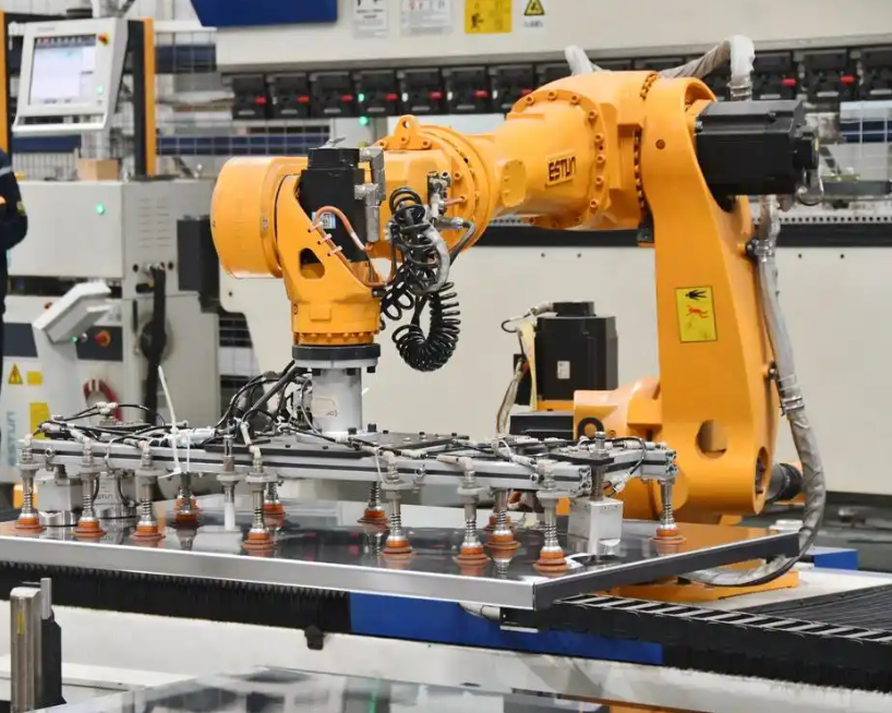
I further analyzed the reversal behavior. Figure 1 is an illustrative representation of the industrial robot used in this study, and it shows the general configuration of the arm and joints. In the measured data, the proposed method reduced the duration of the near-zero velocity dwell. The compensation torque was applied before the velocity sign change, so the joint did not hesitate. The external laser tracker confirmed that the path deviation at the quadrant points was smaller.
The online parameter update also remained stable during the test. The data cleaning logic rejected several current spikes caused by the welding process. Without the cleaning logic, the covariance matrix would have grown, and the compensation torque would have oscillated. With the cleaning logic, the parameter vector converged to a stable set within the first few minutes of operation. The industrial robot then maintained that set throughout the heating cycle.
9. Discussion
The proposed method shows that an industrial robot can achieve significant friction compensation without external torque sensors at every joint. The multi-source data fusion approach uses signals that are already available in most servo systems. The main engineering challenge is not the friction equation itself but the synchronization, cleaning, and timing of the data. A small time misalignment can create a large false acceleration. A single current spike can destabilize the estimator. A few milliseconds of delay can turn a corrective torque into a disturbing torque. I addressed these issues with distributed clock synchronization, dead-zone data cleaning, and look-ahead prediction.
| Design Choice | Benefit for the Industrial Robot | Limitation |
|---|---|---|
| Use of internal servo current | No extra torque sensor | Current-to-torque conversion depends on motor parameters |
| External temperature measurement | Captures thermal drift | Sensor placement affects representativeness |
| Load coupling factor | Adapts to payload changes | Requires a load observer or known payload |
| Recursive least squares | Fast online adaptation | Needs forgetting factor tuning |
| Data cleaning dead zone | Prevents parameter divergence | May ignore legitimate fast events |
| Torque object dictionary mapping | Direct servo access | Depends on drive firmware support |
| Look-ahead prediction | Compensates communication delay | Delay estimate must be accurate |
The method is also compatible with different industrial robot sizes. For a small industrial robot, the friction torque is lower, and the safety limit can be tighter. For a large industrial robot, the thermal time constant is longer, and the temperature sensor placement becomes more important. The same structure applies, but the parameters must be identified for each joint. I recommend a two-stage identification: first, an offline identification of the base friction curve; second, an online update of the thermal and load factors.
Another observation is that the industrial robot should not compensate friction at all speeds with the same aggressiveness. At high speed, the viscous friction is already significant, and the position controller has enough information to follow the path. Overcompensation at high speed can cause vibration. I therefore scale the compensation with a speed-dependent gain. The gain is close to one at low speed and decreases at high speed. This strategy preserves the reversal improvement while avoiding high-speed excitation.
| Speed Region | Compensation Gain | Reason |
|---|---|---|
| Near zero velocity | 1.0 | Compensate static and Coulomb friction |
| Low speed | 1.0–0.8 | Compensate Stribeck transition |
| Medium speed | 0.8–0.5 | Balance viscous and Coulomb effects |
| High speed | 0.5–0.2 | Avoid overcompensation and vibration |
The proposed framework also improves maintenance. Because the industrial robot estimates friction online, a gradual increase in friction can be detected before it becomes a fault. A rising Coulomb term may indicate lubricant degradation or bearing wear. A change in the thermal coefficient may indicate a cooling problem. The same data used for compensation can therefore support condition monitoring. This dual use is valuable in a large welding line where downtime is expensive.
10. Conclusion
I developed a multi-source data fusion method for friction modeling and compensation in an industrial robot. The method extracts a friction residual from servo current and motion data, synchronizes multiple signals with a distributed clock, and updates a temperature-load coupled friction model online. A data cleaning dead zone prevents outliers from corrupting the estimator. The compensation torque is written directly to a servo torque offset object, and a look-ahead prediction compensates for communication delay. A safety limiter protects the industrial robot from abnormal torque commands.
The experimental results on an automotive welding line show that the industrial robot reduces hot-state path error from 0.42 mm to 0.18 mm and improves the process capability index for critical weld characteristics. The method does not require external joint torque sensors, and it uses the existing industrial robot servo and bus infrastructure. The main practical requirements are accurate time synchronization, a reliable temperature measurement point, and access to a torque offset object in the drive. When these conditions are met, the industrial robot can maintain accuracy under variable thermal and load conditions.
Future work can extend the method to multi-joint coupling, where the friction of one joint affects the load of another. Another direction is to combine the friction observer with a thermal model of the entire industrial robot, so that the temperature at unmeasured joints can be estimated. Finally, the same multi-source data fusion framework can be applied to other precision mechanisms, but the industrial robot case shows that online adaptation is essential when the machine operates for long periods under changing conditions.
| Conclusion Item | Result |
|---|---|
| Friction residual extraction | Removes rigid-body dynamics from servo current torque |
| Temperature-load model | Adapts to thermal drift and payload variation |
| Online update | Recursive least squares with data cleaning |
| Servo interface | Direct torque offset through industrial Ethernet |
| Delay handling | Look-ahead velocity prediction |
| Safety | Torque limiting and rate limiting |
| Cold-state RMSE | 0.11 mm |
| Hot-state RMSE | 0.18 mm |
| Weld bead straightness CPK | 1.45 |
| Surface fish-scale uniformity CPK | 1.42 |
In summary, the industrial robot benefits most from friction compensation when the compensation is model-based, online, synchronized, and safely bounded. The multi-source data fusion approach provides a practical path to that goal, and the welding line results confirm its value for high-duty manufacturing.