
The design of mechanical transmission systems often involves a complex interplay between performance, size, weight, and manufacturability. Among advanced transmission technologies, strain wave gear drives, also commonly known as harmonic drives, offer unique advantages such as high reduction ratios in a single stage, compact size, high positional accuracy, and zero-backlash operation. These characteristics make them indispensable in precision fields like robotics, aerospace, and optical instrumentation. However, the very feature that enables their high performance—the controlled elastic deformation of a flexible spline—also introduces significant design complexity. The flexible spline operates under a complex state of cyclical stress, making its longevity and reliability paramount. Traditional design approaches often rely on handbook recommendations and iterative calculations, which may not converge on an optimal solution balancing all competing constraints. This work focuses on formulating the strain wave gear design problem as a formal optimization task, with the explicit goal of minimizing the overall volume (and thus mass) of the transmission, a critical objective for weight-sensitive applications. Crucially, we recognize that a practical design must adhere to manufacturing realities; parameters like gear tooth counts and module sizes are inherently discrete or integer-valued. Treating them as continuous variables yields results that are mathematically elegant but practically unusable without significant, potentially sub-optimal, rounding. Therefore, this paper presents a robust methodology for the mixed discrete variable optimization of strain wave gear systems, employing an enhanced Genetic Algorithm tailored to navigate the discrete, constrained, and non-linear design space effectively.
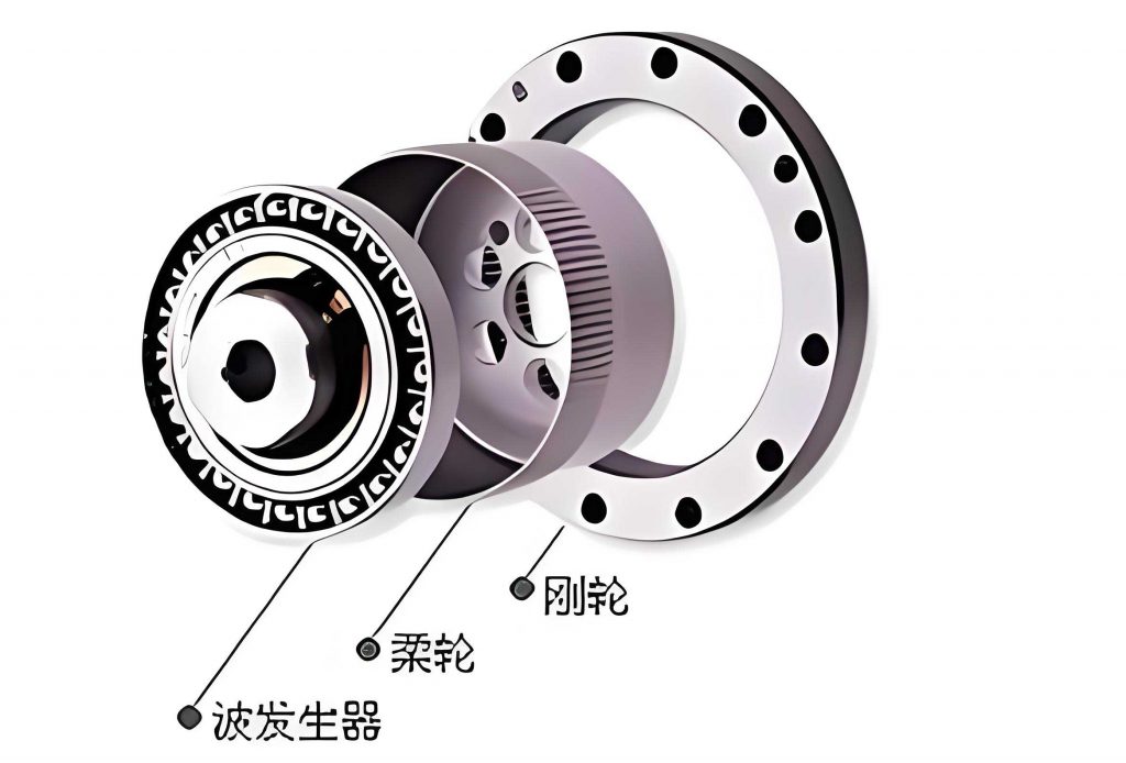
The core principle of a strain wave gear transmission involves three primary components: a rigid circular spline (RS), a flexible spline (FS) with external teeth, and a wave generator (WG). The wave generator, typically an elliptical cam or a set of rotating bearings, is inserted into the flexible spline, causing it to deform elastically into a non-circular shape. This deformation engages the teeth of the flexible spline with those of the rigid spline at two diametrically opposite regions. As the wave generator rotates, the points of engagement travel, resulting in a relative motion between the two splines. The key kinematic relationship is given by the difference in the number of teeth. If the rigid spline has \(Z_G\) teeth and the flexible spline has \(Z_R\) teeth (with \(Z_G > Z_R\)), for each full rotation of the wave generator, the flexible spline rotates backward relative to the rigid spline by \((Z_G – Z_R)\) teeth. The reduction ratio \(i\) for a configuration where the wave generator is the input and the flexible spline is the output, with the rigid spline fixed, is:
$$ i = \frac{Z_R}{Z_G – Z_R} $$
This simple yet profound relationship allows for very high reduction ratios in a compact package. However, the stress state induced in the repeatedly flexing thin-walled cup of the flexible spline is complex, combining bending, torsional, and membrane stresses, which necessitates a rigorous optimization framework to ensure both performance and durability.
Mathematical Model for Mixed Discrete Variable Optimization
To systematically design a strain wave gear for minimum volume, we must first define a quantitative objective function and identify the independent design variables. The primary volume contributors are the flexible spline cup and the gear rim of the rigid circular spline. A simplified yet accurate model for the total volume \(V\) can be derived from their geometries.
Consider a cup-type flexible spline. Its main body is a thin-walled cylinder. Let:
- \(d_{f2}\) be the root diameter of the flexible spline teeth.
- \(L\) be the length of the cylindrical shell of the flexible spline.
- \(h_2\) be the nominal wall thickness of the cylindrical shell.
- \(h_1\) be the wall thickness at the tooth root fillet, often taken as \(h_1 = 2h_2\) for structural reasons.
The volume of the flexible spline cup material can be approximated as that of a cylindrical shell:
$$ V_{FS} \approx \pi L \left[ \left(\frac{d_{f2}}{2} + h_1 + \frac{h_2}{2}\right)^2 – \left(\frac{d_{f2}}{2}\right)^2 \right] $$
Simplifying and using \(h_1 = 2h_2\), we get:
$$ V_{FS} \approx \pi L h_2 (d_{f2} + 3h_2) $$
For the rigid circular spline, modeled as a ring gear, let:
- \(d_G\) be its pitch diameter.
- \(b\) be the face width (gear width).
- \(h_{gf}\) be the total tooth height (typically \(2m\), where \(m\) is the module).
- \(S_G\) be the rim thickness below the tooth root, often specified as \(S_G = k \cdot m\) (with \(k\) between 10 and 20).
The volume of the rigid spline ring is approximately:
$$ V_{RS} \approx \pi b \left[ \left(\frac{d_G}{2} + h_{gf} + S_G\right)^2 – \left(\frac{d_G}{2}\right)^2 \right] = \pi b (h_{gf} + S_G) d_G $$
Now, we relate these dimensions to fundamental gear parameters and the wave generator. For a standard strain wave gear:
$$ d_G = m Z_G, \quad d_R = m Z_R $$
The wave generator produces a radial deflection \(w_0\), approximately equal to half the wave height \(d\), which is itself related to the module: \(d \approx 2m\). The flexible spline root diameter is:
$$ d_{f2} = d_R – \frac{9}{8}d = m Z_R – \frac{9}{4}m = m\left(Z_R – \frac{9}{4}\right) $$
Substituting all relationships into the total volume expression \(V = V_{FS} + V_{RS}\) and using standard values \(h_{gf}=2m\), \(S_G=20m\), we obtain the final objective function \(f(\mathbf{x})\):
$$ f(\mathbf{x}) = \pi L h_2 \left[ m\left(Z_R – \frac{9}{4}\right) + 3h_2 \right] + 22 \pi b m^2 Z_G $$
$$ f(\mathbf{x}) = \pi \left\{ L h_2 \left[ m Z_R – \frac{9}{4}m + 3h_2 \right] + 22 b m^2 Z_G \right\} $$
The constant \(\pi\) can be omitted for optimization purposes without affecting the location of the optimum. Therefore, our minimization objective becomes:
$$ \text{Minimize: } f(\mathbf{x}) = L h_2 \left( m Z_R – \frac{9}{4}m + 3h_2 \right) + 22 b m^2 Z_G $$
The design vector \(\mathbf{x}\) comprises six variables, each with distinct characteristics relevant to manufacturing:
$$ \mathbf{x} = [x_1, x_2, x_3, x_4, x_5, x_6]^T = [Z_G, Z_R, m, L, b, h_2]^T $$
- \(Z_G, Z_R\): Tooth counts for the rigid and flexible splines. These must be integers. Furthermore, for a two-wave generator, they must differ by a small, even number (commonly 2) to achieve the desired kinematic effect and ensure proper meshing.
- \(m\): Module. This is a non-equally spaced discrete variable, as it must be selected from a standardized series of preferred values (e.g., 0.2, 0.25, 0.3, 0.4, 0.5, 0.6, 0.8, 1.0… mm).
- \(L, b\): Length and face width. While conceptually continuous, for practical engineering drawings and machining, these are typically specified as integers (in mm).
- \(h_2\): Flexible spline wall thickness. This is a continuous variable. However, from a manufacturing and quality control perspective, it is reasonable to control its precision, for example, to one-tenth of a millimeter.
This combination makes the strain wave gear optimization problem a genuine mixed discrete variable optimization challenge, which cannot be accurately solved by standard continuous-variable methods.
Constraint Formulation
A feasible strain wave gear design must satisfy a multitude of constraints related to strength, geometry, kinematics, and manufacturability.
1. Flexible Spline Strength Constraint
The flexible spline is subjected to a complex, multiaxial, cyclical stress state during operation. The primary stress components are:
- Bending Stresses (\( \sigma_z, \sigma_\theta \)): Caused by the radial deflection imposed by the wave generator. The circumferential bending stress \(\sigma_\theta\) is particularly significant.
- Torsional Shear Stress (\( \tau_{zu} \)): Arises from transmitting the torque through the thin-walled cylinder.
- Pure Torsional Shear Stress (\( \tau_m \)): Due to the output torque load.
Based on elasticity theory and empirical correction factors, these stresses can be calculated as follows:
$$ \sigma_z = K_M K_d C_R \frac{M_z}{W} = K_M K_d C_R \frac{w_0 E h_2}{r_m^2} $$
$$ \sigma_\theta = K_M K_d C_R \frac{w_0 E h_2}{r_m^2} \quad \text{(Note: often } \sigma_\theta \text{ is the dominant bending stress)} $$
$$ \tau_{zu} = K_M K_d C_S \frac{M_{zu}}{J} = K_M K_d C_S \frac{w_0 E h_2}{r_m L} $$
$$ \tau_m = K_u K_d \frac{M_1}{2\pi h_2 r_m^2} $$
where:
- \(w_0\) is the maximum radial displacement (\(\approx m\)).
- \(E, \nu\) are Young’s modulus and Poisson’s ratio of the FS material.
- \(r_m\) is the mean radius of the FS cylindrical shell.
- \(M_1\) is the output torque.
- \(K_M, K_d, K_u, C_R, C_S\) are correction factors for load distribution, dynamic effects, and geometry.
The stress amplitudes (\(\sigma_a, \tau_a\)) and mean stresses (\(\sigma_m, \tau_m\)) for fatigue analysis are:
$$ \sigma_a = \sigma_\theta, \quad \sigma_m = 0 $$
$$ \tau_a = \tau_m = 0.5(\tau_m + \tau_{zu}) $$
The safety factors for bending (\(S_\sigma\)) and shear (\(S_\tau\)), based on the Soderberg or Goodman criterion, are:
$$ S_\sigma = \frac{\sigma_{-1}}{K_\sigma \sigma_a + \psi_\sigma \sigma_m} = \frac{\sigma_{-1}}{K_\sigma \sigma_a} $$
$$ S_\tau = \frac{\tau_{-1}}{K_\tau \tau_a + \psi_\tau \tau_m} $$
where \(\sigma_{-1}, \tau_{-1}\) are the fully reversed bending and shear endurance limits, and \(K_\sigma, K_\tau\) are the fatigue stress concentration factors. The combined safety factor \(S\) for multi-axial fatigue is computed using an interactive theory (e.g., von Mises with mean stress correction):
$$ S = \frac{S_\sigma S_\tau}{\sqrt{S_\sigma^2 + \xi S_\tau^2}} \geq [S] $$
where \(\xi\) is an interaction factor (often 1.0 for von Mises), and \([S]\) is the required minimum safety factor (e.g., 1.5 for reliable operation).
2. Meshing and Non-Interference Constraints
To ensure smooth power transmission and avoid tooth tip digging, the meshing process must be analyzed. The fundamental condition is that the tooth engagement must begin and end cleanly without the tip of one gear interfering with the flank of the other. This is expressed through an inequality on the engagement angles. Let \(\theta_{L1}\) be the angular distance on the rigid spline from the start of active profile to the tooth tip, and \(\theta_{L2}\) be the corresponding angular distance on the flexible spline to its tooth tip. The non-interference condition is:
$$ \theta_{L1} – \theta_{L2} \geq 0 $$
These angles depend on the pressure angle (\(\alpha\)), addendum (\(h_a\)), dedendum (\(h_f\)), working pressure angle, and the specific tooth profile modifications used in strain wave gears. Their detailed derivation involves the geometry of conjugate action under deflection.
3. Kinematic (Transmission Ratio) Constraint
This is an equality constraint that must be satisfied exactly. For a given target reduction ratio \(i\), with the wave generator as input and the flexible spline as output:
$$ Z_R – i (Z_G – Z_R) = 0 \quad \text{or} \quad \frac{Z_R}{Z_G – Z_R} – i = 0 $$
In practice, for a two-wave generator, \(Z_G – Z_R = 2\) is typical. Therefore, this constraint often simplifies to ensuring the tooth difference is correct for the desired ratio.
4. Geometric and Practical Bounds
Based on design experience and handbooks, reasonable bounds are imposed to ensure a practical, manufacturable design:
$$
\begin{aligned}
0.8 \, d_R &\leq L \leq 1.2 \, d_R \\
0.2 \, d_R &\leq b \leq 0.25 \, d_R \\
0.01 \, d_R &\leq h_2 \leq 0.015 \, d_R \\
180 &\leq Z_G \leq 230 \\
Z_G – 2 &\leq Z_R \leq Z_G – 2 \quad \text{(for a fixed difference of 2)}
\end{aligned}
$$
Additionally, if profile shifting (x-modification) is applied, constraints to prevent undercut, excessive tooth thinning, and root fillet interference must be included.
The complete optimization problem is summarized as:
$$
\begin{aligned}
& \underset{\mathbf{x}}{\text{minimize}}
& & f(\mathbf{x}) = L h_2 \left( m Z_R – \frac{9}{4}m + 3h_2 \right) + 22 b m^2 Z_G \\
& \text{subject to}
& & g_1(\mathbf{x}): S – [S] \geq 0 \quad \text{(Strength)} \\
& & & g_2(\mathbf{x}): \theta_{L1} – \theta_{L2} \geq 0 \quad \text{(Non-interference)} \\
& & & h_1(\mathbf{x}): Z_R / (Z_G – Z_R) – i = 0 \quad \text{(Kinematic)} \\
& & & g_{3-8}(\mathbf{x}): \text{Geometric bounds on } L, b, h_2, Z_G, Z_R \\
& & & \mathbf{x} \in \mathbb{X}, \quad \mathbb{X} = \mathbb{Z}^2 \times \mathbb{D}_m \times \mathbb{Z}^2 \times \mathbb{R}_{h_2}
\end{aligned}
$$
where \(\mathbb{D}_m\) is the discrete set of standard modules, and \(\mathbb{R}_{h_2}\) is the continuous space for \(h_2\).
An Enhanced Hybrid Genetic Algorithm for Mixed Discrete Variables
Genetic Algorithms (GAs) are population-based stochastic search methods inspired by natural selection. They are well-suited for complex, non-convex, and mixed-variable problems because they work on a coding of the variables, not the variables themselves, and require no gradient information. However, a standard GA with continuous operators is ill-equipped to handle the discrete nature of key strain wave gear design variables. We propose an enhanced Hybrid Genetic Algorithm (HGA) with specific modifications for this purpose.
1. Chromosome Representation and Fitness Evaluation
We employ real-number encoding, where each chromosome is a vector of the six design variables \(\mathbf{x}\). This is more natural and efficient for numerical optimization compared to binary encoding.
To handle constraints, an exact penalty function method is used to construct a new, unconstrained objective function \(\Phi(\mathbf{x}, \mathbf{r})\):
$$ \Phi(\mathbf{x}, \mathbf{r}) = f(\mathbf{x}) + \sum_{j=1}^{p} r_j \cdot \max[0, -g_j(\mathbf{x})]^2 + \sum_{k=1}^{q} \rho_k \cdot |h_k(\mathbf{x})| $$
where \(r_j\) and \(\rho_k\) are penalty coefficients that are progressively increased over generations to force feasibility. The fitness function \(F_i\) for chromosome \(i\) in a population of size \(P\) is then scaled from this penalized objective to ensure positive values for selection:
$$ F_i = C_{max} – \Phi(\mathbf{x}_i, \mathbf{r}), \quad i=1,…,P $$
where \(C_{max}\) is the maximum \(\Phi\) value in the current population.
2. Core Genetic Operators
- Selection: A roulette-wheel (fitness-proportional) selection is used, giving higher-probability mating chances to fitter individuals.
- Crossover: A blend crossover (BLX-α) operator for real-coded GAs is applied to the continuous representation of variables. For two parent vectors \(\mathbf{x}^1\) and \(\mathbf{x}^2\), an offspring \(\mathbf{x}^{new}\) is generated as:
$$ x^{new}_j = x^1_j + \gamma_j (x^2_j – x^1_j) $$
where \(\gamma_j\) is a random number uniformly distributed in \([-0.5, 1.5]\) for a typical BLX-0.5. This encourages exploration. - Mutation: A non-uniform mutation operator is applied. For a variable \(x_j\) with bounds \([L_j, U_j]\), the mutated value \(x’_j\) is:
$$ x’_j = \begin{cases}
x_j + \Delta(t, U_j – x_j) & \text{if a random digit is 0}\\
x_j – \Delta(t, x_j – L_j) & \text{if a random digit is 1}
\end{cases} $$
where \(\Delta(t, y) = y \cdot (1 – r^{(1-t/T)^\eta})\), \(r\) is random in [0,1], \(t\) is the current generation, \(T\) is the maximum generation, and \(\eta\) is a shape parameter. This allows larger jumps early and finer tuning later. - Elitism: The best chromosome from each generation is guaranteed to survive to the next, preserving found gains.
3. Key Enhancement: Engineering-Driven Variable Discretization
This is the crucial step that tailors the GA to the mixed discrete problem. After every application of crossover and mutation, the offspring’s variables are processed according to their type before fitness evaluation.
For Integer Variables (\(Z_G, Z_R, L, b\)): The raw real value \(x_j^{real}\) is simply rounded to the nearest integer.
$$ x_j^{int} = \text{round}(x_j^{real}) $$
For Non-Equally Spaced Discrete Variables (module \(m\)): Let the set of standard modules be \(M = \{m_1, m_2, …, m_v\}\). The algorithm finds the interval \([m_i, m_{i+1}]\) containing the raw value \(x_m^{real}\). The discrete value is assigned by nearest-neighbor rounding:
$$ x_m^{disc} = \begin{cases}
m_i & \text{if } |x_m^{real} – m_i| \le |x_m^{real} – m_{i+1}| \\
m_{i+1} & \text{otherwise}
\end{cases} $$
For “Continuously Valued” Engineering Variables (wall thickness \(h_2\)): While mathematically continuous, manufacturing tolerances dictate a practical resolution (e.g., 0.1 mm). Therefore, we process it to a specified number of decimal places \(w\):
$$ h_2^{eng} = \frac{\text{round}(h_2^{real} \times 10^w)}{10^w} $$
This “engineering quantization” is performed during the optimization loop, ensuring the algorithm searches the space of practically acceptable values, and the final result requires no post-processing.
4. Key Enhancement: Chaos-Immigration Operator for Diversity
A common pitfall of GAs is premature convergence to a local optimum. To maintain population diversity, we introduce a Chaos-Immigration Operator. Every \(K\) generations (e.g., \(K=10\)), a fraction of the worst-performing individuals are replaced by “immigrants” generated using a chaotic sequence. Chaotic maps, like the logistic map, produce ergodic, non-periodic sequences that can efficiently explore the design space.
$$ z_{n+1} = \mu z_n (1 – z_n), \quad z_n \in (0, 1), \mu=4 $$
A chaotic variable \(z\) is mapped to a design variable within its bounds:
$$ x_j^{chaos} = L_j + z^{(j)} \cdot (U_j – L_j) $$
These chaotic vectors are then subjected to the same engineering-driven discretization process described above before being inserted into the population. This operator acts as a powerful macro-mutation, injecting fresh genetic material and helping the algorithm escape local attractors.
The flowchart of the proposed Enhanced Hybrid Genetic Algorithm (EHGA) for strain wave gear optimization is as follows:
- Initialize: Generate a random initial population of size \(P\). Apply discretization/engineering rounding to all individuals. Evaluate fitness.
- Main Loop (for \(t = 1\) to \(T_{max}\)):
- Select parents via roulette wheel.
- Apply BLX-α crossover and non-uniform mutation to create offspring.
- Apply Engineering Discretization to all offspring variables.
- Evaluate fitness of new offspring.
- Combine parents and offspring, apply elitism to form the new population.
- If (t mod \(K == 0\)): Apply Chaos-Immigration operator (replace worst individuals with discretized chaotic vectors).
- Terminate: Output the best individual found as the optimal design.
Optimization Design Case Study
To demonstrate the effectiveness of the proposed method, we consider the design of a single-stage strain wave gear speed reducer with the following specifications:
- Transmission Ratio (\(i\)): 100
- Output Torque (\(M_1\)): 500 Nm
- Input Speed: 3000 rpm
- Operating Condition: 8-10 hours daily, smooth load.
- Flexible Spline Material: 40CrNiMoA alloy steel with endurance limits \(\sigma_{-1} = 500\) MPa, \(\tau_{-1} = 250\) MPa.
Algorithm Parameters:
- Population Size (\(P\)): 50
- Maximum Generations (\(T_{max}\)): 500
- Crossover Probability: 0.6
- Mutation Probability: 0.06
- Immigration Interval (\(K\)): 10 generations
- Immigration Rate: 20% of population (replace 10 worst individuals)
- Engineering Precision for \(h_2\) (\(w\)): 1 (i.e., 0.1 mm resolution)
- Standard Module Set (\(m\)): {0.2, 0.25, 0.3, 0.4, 0.5, 0.6, 0.8, 1.0} mm
The EHGA was implemented, and the optimization was performed. For comparison, a standard continuous-variable GA (without discretization or immigration) was also run on the same problem, treating all variables as continuous real numbers.
Results and Discussion
The optimal design parameters obtained from both approaches are summarized in the table below. The objective function value \(f(\mathbf{x})\) is proportional to volume.
| Design Variable / Result | Proposed EHGA (Mixed Discrete) | Standard GA (Continuous) | Notes on Practicality |
|---|---|---|---|
| Rigid Spline Teeth (\(Z_G\)) | 202 | 199.0906 | Integer required for manufacture. Continuous result is unusable. |
| Flexible Spline Teeth (\(Z_R\)) | 200 | 197.1194 | Integer required. Difference (\(Z_G-Z_R=2\)) is correct for ratio i=100. |
| Module (\(m\)) [mm] | 0.5 | 0.5082 | Must be a standard value. 0.5 mm is a standard module; 0.5082 is not. |
| Flex. Spline Length (\(L\)) [mm] | 118 | 120.1909 | Typically an integer dimension on a drawing. |
| Face Width (\(b\)) [mm] | 20 | 20.0466 | Typically an integer dimension. |
| Wall Thickness (\(h_2\)) [mm] | 1.0 | 1.0064 | EHGA respects 0.1 mm precision. Continuous value is over-specified. |
| Objective \(f(\mathbf{x})\) [proportional to mm³] | 105,347.81 | 106,866.79 | The EHGA found a better, manufacturable solution. |
| Safety Factor (\(S\)) | > 1.5 (Feasible) | > 1.5 (Feasible) | Both satisfy the strength constraint. |
| Manufacturing Readiness | Directly usable | Requires rounding/post-processing | Rounding continuous results may violate constraints or be sub-optimal. |
The results clearly illustrate the superiority and practical necessity of the mixed-discrete approach. The standard continuous GA produced a mathematically optimized but physically unrealizable set of parameters: non-integer tooth counts, a non-standard module, and overly precise dimensions. Manually rounding these values to the nearest practical ones (e.g., \(Z_G=199\), \(Z_R=197\), \(m=0.5\)) would not only potentially degrade performance but could also violate critical constraints like the exact transmission ratio or the strength requirement. In contrast, the proposed Enhanced Hybrid Genetic Algorithm searched directly within the space of manufacturable values. It successfully found a combination of standard modules, integer tooth counts and dimensions, and a sensibly quantized wall thickness that simultaneously minimizes volume and satisfies all engineering constraints. Remarkably, the objective function value for this manufacturable design is actually lower than that of the continuous optimum, demonstrating that the true global optimum for this class of problems often lies on the discrete grid of practical values, not in the continuous relaxation.
The evolution of the best objective function value over generations showed that the chaos-immigration operator effectively prevented stagnation. Periodic injections of chaotic individuals provided renewed diversity, enabling the algorithm to explore different regions of the discrete landscape and converge to a robust solution.
Conclusion
This work presented a comprehensive methodology for the optimal design of strain wave gear transmissions, explicitly addressing the mixed-integer and discrete nature of real-world design parameters. By formulating a detailed nonlinear programming model with objectives and constraints for strength, kinematics, and geometry, we captured the essential engineering trade-offs. The primary contribution is the development of an Enhanced Hybrid Genetic Algorithm (EHGA) that integrates two key innovations: 1) an engineering-driven discretization step embedded within the evolutionary loop, which ensures all design variables conform to manufacturing standards throughout the search process, and 2) a chaos-immigration operator that preserves population diversity and enhances global convergence capability.
The case study for a high-ratio, high-torque reducer demonstrated the algorithm’s efficacy. The EHGA successfully located an optimal design comprising standard modules and integer dimensions that is directly applicable to manufacturing without any need for post-processing or ad-hoc rounding—a significant advantage over traditional continuous optimization approaches. The final design met all stringent performance constraints, including fatigue safety and meshing quality, while achieving a minimal volume. This approach provides a powerful, practical, and automated tool for engineers designing compact and efficient strain wave gear drives for advanced mechanical systems, bridging the gap between theoretical optimization and production-ready engineering design.
Future work may extend this framework to multi-objective optimization, considering additional goals such as maximizing efficiency, minimizing instantaneous elastic backlash, or optimizing torsional stiffness. The integration of more detailed finite element analysis results for stress calculation within the optimization loop could further enhance accuracy, albeit at a higher computational cost. The core EHGA strategy, however, is broadly applicable to a wide range of mixed discrete-continuous optimization problems in mechanical design.