Optimizing RV Reducer Structure Using a Discrete Shuffled Frog Leaping Algorithm

As a core component driving joint motion in industrial robots, the RV reducer is prized for its high transmission efficiency, substantial load-bearing capacity, and minimal backlash. Its widespread adoption underscores its critical role. However, due to a relatively late start in development, immature design theories and production processes, and high manufacturing costs domestically, many robotics enterprises still rely on importing high-performance RV reducers from abroad. This dependency highlights the paramount importance of optimizing and improving the structural design of domestic RV reducers. Consequently, numerous scholars have dedicated research efforts to this area. For instance, some researchers have employed genetic algorithms and NSGA-II algorithms to pursue optimization goals centered on maximizing overall efficiency and minimizing volume. Others have conducted multi-objective optimization targeting the volume and efficiency of RV reducers based on genetic algorithms. Further studies have focused on enhancing the load-bearing capacity through traditional combined tooth profile modification methods for cycloidal gears, establishing mathematical models for modification amount search and solving them using grid methods. While these contributions have significantly advanced RV reducer parameter design, they often involve manual rounding of results and may not achieve the highest possible precision. Therefore, this paper attempts to apply a novel swarm intelligence algorithm, aiming to further refine the parameters of the RV reducer and enhance its overall performance based on the foundation laid by prior research.

The Shuffled Frog Leaping Algorithm (SFLA), a modern heuristic bio-inspired swarm intelligence optimization algorithm, is known for its conceptual simplicity, fast computation, and excellent problem-solving and global search capabilities. It has been widely applied to practical engineering problems such as water resource allocation, bridge pier maintenance, and workshop scheduling. This paper proposes a new method for the single-objective volume optimization of RV reducers based on a Discrete Shuffled Frog Leaping Algorithm (D-SFLA). The goal is to achieve further structural improvements under the premise of satisfying constraints regarding overall stiffness, strength, and transmission efficiency, enabling the RV reducer’s application in spatially demanding scenarios.

Mathematical Model for RV Reducer Structural Optimization

Structural Principles

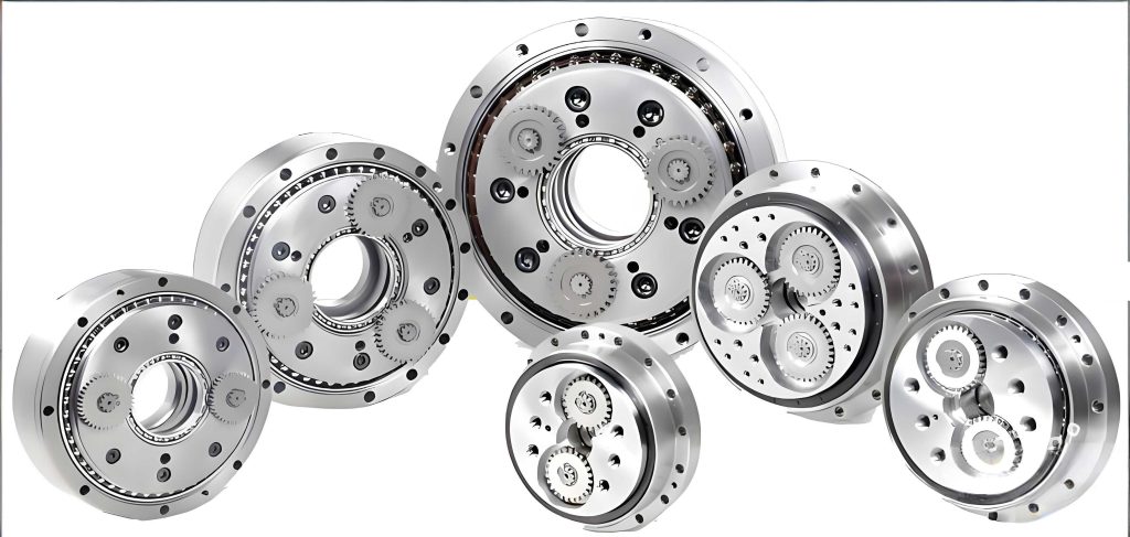
The RV reducer is a closed differential gear train, structurally divided into two stages. The differential stage consists of an input shaft, a sun gear, planetary gears, and a planet carrier (arm). The closed stage is a cycloidal pin-wheel planetary transmission mechanism comprising crankshafts, cycloidal gears, pins/pin teeth, and a pin housing. If the pin housing is fixed, the planet carrier acts as the output member; if the planet carrier is fixed, the pin housing serves as the output. This paper selects the pin housing as the output member.

Mathematical Modeling

The volume of the RV reducer is primarily determined by the dimensions of its first-stage involute gear transmission and its second-stage cycloidal drive. To mitigate the forces between the cycloidal gears and the crankshafts in the second stage, the center distance of the first-stage gear transmission is required to be slightly larger than one-quarter of the pin gear center circle diameter of the second stage. Since the volume occupied by the gear transmission is approximately linearly positively correlated with its center distance, we define the first-stage gear transmission center distance as the objective function, denoted as $f(\mathbf{X})$, and establish a mathematical model to minimize it.

Given the known input-output requirements and total transmission ratio of the RV reducer, the independent design variables are:

$$\mathbf{X} = [x_1, x_2, x_3] = [z_1, z_2, m]$$

where $z_1$ is the sun gear tooth number, $z_2$ is the planetary gear tooth number, and $m$ is the standard spur gear module.

Based on mechanical design literature, the following constraints must be satisfied:

Undercutting Avoidance: To prevent root undercutting of the pinion (sun gear):
$$g_1(\mathbf{X}) = 17 – z_1 \le 0$$
Transmission Ratio Constraint: To fully utilize the advantages of high torque capacity and smooth load transmission in the second cycloidal stage, the gear ratio $i_1$ of the first stage should not be too small:
$$g_2(\mathbf{X}) = 1.5 – i_1 \le 0$$
where $i_1 = z_2 / z_1$.
Bending Fatigue Strength: To satisfy tooth bending fatigue strength for the pinion:
$$g_3(\mathbf{X}) = m – \sqrt[3]{\frac{2 K T_1 Y_{Fa} Y_{Sa}}{\phi_d z_1^2 [\sigma_F]}} \le 0$$
where $m$ is selected from the first series of standard modules, $K$ is the load factor, $Y_{Fa}$ is the form factor, $Y_{Sa}$ is the stress correction factor, $\phi_d$ is the face width coefficient, $[\sigma_F]$ is the allowable bending stress, and $T_1$ is the torque transmitted by the sun gear:
$$T_1 = \frac{9.55 \times 10^6 P}{n i}$$
with $n$ as the rated output speed and $i$ as the total RV reducer ratio.
Contact Fatigue Strength: The first-stage planetary gear transmission must satisfy surface contact fatigue strength:
$$g_4(\mathbf{X}) = m z_1 – 2.32 \sqrt[3]{\frac{K T_1 (i_1+1)}{\phi_d i_1} \left( \frac{Z_E}{[\sigma_H]} \right)^2} \le 0$$
where $Z_E$ is the elasticity coefficient and $[\sigma_H]$ is the allowable contact stress.
Adjacency Condition: For two adjacent planetary gears, their center distance must be greater than their tip diameters to avoid interference (let $n_p$ be the number of planets):
$$g_5(\mathbf{X}) = (z_1 + z_2)\sin(\pi / n_p) – (z_2 + 2h_a^*) < 0$$
where $h_a^*$ is the addendum coefficient.
Structural Balance: To ensure structural harmony, the maximum diameter of the involute planetary stage should be close to that of the cycloidal stage:
$$g_6(\mathbf{X}) = 0.9 r_p – m(z_1/2 + z_2) \le 0$$
$$g_7(\mathbf{X}) = m(z_1/2 + z_2) – 1.1 r_p \le 0$$
where $r_p$ is the pin gear center circle radius, calculated as:
$$r_p = (0.85 \sim 1.3) (2T / [\tau])^{1/3}$$
and $T$ is the output torque:
$$T = \frac{9.55 \times 10^6 P \eta}{n}$$
with $\eta$ as the total transmission efficiency, which should be no less than 85% in practice.
Center Distance Constraint: To improve bearing load conditions on the crankshaft, the center distance should be constrained relative to the second-stage size:
$$g_8(\mathbf{X}) = 0.5 r_p – m(z_1 + z_2)/2 \le 0$$
$$g_9(\mathbf{X}) = m(z_1 + z_2)/2 – 0.6 r_p \le 0$$

Denoting the constraint functions as $g_i(\mathbf{X})$ for $i=1,\ldots,9$, the complete nonlinear constrained optimization model for the RV reducer is:

$$
\begin{aligned}
\min \quad & f(\mathbf{X}) = \frac{m(z_1 + z_2)}{2} \\
\text{subject to} \quad & g_i(\mathbf{X}) \le 0, \quad i = 1, 2, \ldots, 9
\end{aligned}
$$

Introduction to the Discrete Shuffled Frog Leaping Algorithm

Standard SFLA Fundamentals

The Shuffled Frog Leaping Algorithm is a memetic meta-heuristic inspired by the foraging behavior of frogs. Imagine a population of frogs, each representing a potential solution (its position) to an optimization problem, with its fitness determined by the proximity to the food source (the optimal solution). The population is divided into several parallel “memeplexes” (subgroups). Within each memeplex, frogs evolve through a local search process: the worst frog learns from the best frog in its own memeplex and from the globally best frog, adjusting its position (solution) accordingly. After a predefined number of local evolution steps, all memeplexes are shuffled and recombined to share global information. This process of partitioning, local evolution, and shuffling continues until a termination criterion is met. The standard SFLA procedure is as follows:

Parameter Definition: Define key parameters: number of memeplexes $m$, frogs per memeplex $p$, total population size $U = m \times p$, maximum number of local evolution steps per memeplex $L_{\max}$, maximum number of global shuffling iterations $G_{\max}$, and sub-memeplex size $q$.
Population Initialization: Randomly generate $U$ frog positions (solutions) within the feasible domain. Evaluate their fitness and sort the population. Identify the global best frog $U_g$.
Memeplex Formation & Local Evolution: Partition the sorted population into $m$ memeplexes. For each memeplex, identify the worst frog $U_w$ and the best frog $U_b$. For $L_{\max}$ steps, attempt to improve $U_w$ using the update rule:
$$D = rand() \times (U_b – U_w)$$
$$U_w^{\text{new}} = U_w + D, \quad \text{with } |D| \le D_{\max}$$
where $D_{\max}$ is the maximum allowed leap. If $U_w^{\text{new}}$ is better, replace $U_w$. If not, repeat the process using $U_g$ instead of $U_b$. If still no improvement, replace $U_w$ with a randomly generated solution.
Shuffling and Termination: After local evolution in all memeplexes, shuffle all frogs back into one population, re-sort, and update $U_g$. Check if $G_{\max}$ is reached. If yes, terminate; otherwise, return to Step 3.

Discretization of SFLA

To handle optimization problems with discrete variables, such as the RV reducer design where gear teeth numbers and module are discrete, the standard continuous SFLA requires adaptation into a Discrete SFLA (D-SFLA):

Discrete Encoding: Each discrete variable is assigned a unique index from its feasible set. A solution (frog) is represented by a vector of these indices. Initialization involves randomly selecting indices for each dimension.
Index-based Operations: Before the local update, the positions of the global best $U_g$, memeplex best $U_b$, and memeplex worst $U_w$ are converted to their corresponding index vectors $U_{gs}$, $U_{bs}$, and $U_{ws}$.
Discrete Update Strategy: The leap operation is performed on the index space and then rounded to the nearest valid integer index to ensure the result remains discrete. The update rule is modified as:
$$S_s = \begin{cases}
\min(\text{round}(r_1 \times (U_{bs} – U_{ws})), S_{\max}) & \text{if } U_{bs} – U_{ws} \ge 0 \\
\max(\text{round}(r_2 \times (U_{bs} – U_{ws})), -S_{\max}) & \text{if } U_{bs} – U_{ws} < 0
\end{cases}$$
$$U_{ws}’ = U_{ws} + S_s$$
where $S_s$ is the discrete step, $r_1, r_2$ are random numbers in [0,1], $S_{\max}$ is the maximum step size in index units, and $\text{round()}$ ensures an integer step. The new index vector $U_{ws}’$ is then converted back to actual variable values for fitness evaluation. Other algorithm steps remain conceptually similar to the standard SFLA.

Optimization Case Study Based on D-SFLA

RV Reducer Design Parameters

The optimization is performed for an RV-450E type reducer with the following specifications: Total transmission ratio $i = 81$, output speed $n = 5 \, \text{rpm}$, input power $P = 4.28 \, \text{kW}$. First-stage gears are made from 20Cr (case-hardened). The following parameters are obtained from mechanical handbooks and literature: Load factor $K = 1.10$, form factor $Y_{Fa} = 2.91$, stress correction factor $Y_{Sa} = 1.53$, face width coefficient $\phi_d = 0.3$, total efficiency $\eta = 0.88$, allowable bending stress $[\sigma_F] = 640 \, \text{MPa}$, allowable contact stress $[\sigma_H] = 1800 \, \text{MPa}$, elasticity coefficient $Z_E = 189.9 \, \text{MPa}^{1/2}$, number of planets $n_p = 3$, and addendum coefficient $h_a^* = 1$.

Fitness Function Construction via Penalty Method

Swarm intelligence algorithms typically require an unconstrained fitness function. The RV reducer model involves nonlinear inequality constraints $g_i(\mathbf{X}) \le 0$. We employ an exterior penalty function method to transform the constrained problem. The fitness function $F(\mathbf{X}, M)$ is defined as:

$$F(\mathbf{X}, M) = f(\mathbf{X}) + M \sum_{i=1}^{9} \left[ \max(g_i(\mathbf{X}), 0) \right]^2$$

where $M$ is a sufficiently large penalty factor. Minimizing $F(\mathbf{X}, M)$ approximates minimizing $f(\mathbf{X})$ while satisfying all constraints. This $F(\mathbf{X}, M)$ serves as the fitness function for the D-SFLA.

Algorithm Parameter Settings

For a fair comparison with Particle Swarm Optimization (PSO) and a Genetic Algorithm (GA), termination for all three algorithms is set at reaching the maximum global iterations. Common parameters are: $L_{\max}=40$, $G_{\max}=200$, problem dimension $D=3$, total population/particles $U=400$. The discrete variable bounds are set as: $z_1 \in \{17, 18, \ldots, 71\}$, $z_2 \in \{27, 28, \ldots, 101\}$, and $m$ belongs to the first series of standard modules $\{0.2, 0.25, \ldots, 20\}$.

D-SFLA: Memeplex count $m=20$, frogs per memeplex $p=20$, sub-memeplex size $q=15$, step length coefficient $L_{st}=0.5$.
PSO: Inertia weight $w=0.9$, cognitive and social learning factors $c_1 = c_2 = 2$, velocity limits $v_{\max}=1, v_{\min}=-1$. The standard PSO update equations are used:
$$v_{k+1} = w v_k + c_1 r_1 (p_{\text{best}} – x_k) + c_2 r_2 (g_{\text{best}} – x_k)$$
$$x_{k+1} = x_k + v_{k+1}$$
GA: Implemented using MATLAB’s toolbox with equivalent population size and generation limits.

Optimization Results and Comparative Analysis

Each algorithm (D-SFLA, PSO, GA) was run independently 20 times under the same conditions. The results from PSO and GA were manually rounded to the nearest feasible discrete values. The optimal solution obtained using MATLAB’s `fmincon` function (for the continuous problem, subsequently rounded) from a referenced study is also included for baseline comparison. The comparative results are summarized in the table below.

Algorithm	Objective Value $f(\mathbf{X})$	Design Variables $(z_1, z_2, m)$	Mean $f(\mathbf{X})$	Variance
D-SFLA	69.0	(18, 27, 3)	69.75	1.54
PSO (Rounded)	72.0	(18, 30, 3)	77.75	2.66
GA (Rounded)	72.0	(27, 45, 2)	76.06	11.28
fmincon (Rounded)	79.5	(18, 35, 3)	–	–

The results clearly demonstrate the effectiveness of the swarm intelligence approaches. The D-SFLA achieved the best (minimum) center distance of 69.0 mm, which is approximately 13.2% lower than the 79.5 mm obtained by the traditional `fmincon` approach. Even the worst solution found by D-SFLA in 20 runs (73.5 mm) is comparable to the best solutions found by PSO and GA (72.0 mm). Furthermore, D-SFLA exhibits the lowest mean and variance among the swarm algorithms, indicating not only higher solution quality but also superior stability and robustness, with a lower tendency to get trapped in local optima. Critically, the D-SFLA inherently operates in the discrete space, eliminating the need for post-optimization manual rounding, which enhances the credibility and scientific rigor of the result.

The convergence characteristics of the D-SFLA are illustrated by plotting the best, worst, and average fitness values over iterations from the 20 runs. The curves show that the algorithm converges rapidly, with solutions stabilizing within the first 10-20 generations. This demonstrates the D-SFLA’s fast convergence speed for this RV reducer volume optimization problem.

Conclusion

This paper successfully applied a Discrete Shuffled Frog Leaping Algorithm to the single-objective volume minimization problem of an RV reducer. The D-SFLA inherently handles discrete design variables, producing feasible, directly applicable results without requiring manual rounding. The optimization results significantly outperform those obtained by a traditional nonlinear constraint solver (`fmincon`). In comparative tests with other prominent swarm intelligence algorithms, namely PSO and GA, the D-SFLA proved superior in terms of solution precision, convergence speed, global search capability, and result stability. These advantages establish the Discrete Shuffled Frog Leaping Algorithm as a highly effective and reliable new method for solving discrete variable optimization problems in complex mechanical system design, such as the structural optimization of RV reducers.