
In the realm of robotics, the pursuit of adaptability and resilience in complex environments has led to the emergence of self-reconfigurable modular robots. These systems, composed of multiple identical unit modules, possess the inherent ability to autonomously alter their configurations and operational postures, making them exceptionally suited for tasks such as field exploration, search and rescue in confined spaces, and pipeline inspection. Among the various forms these robots can assume, the bionic robot, particularly those mimicking legged locomotion, stands out due to its potential for traversing uneven terrain. In this work, I delve into the design and analysis of a novel self-reconfigurable bionic quadruped robot, constructed from ten identical unit modules. The primary focus is on establishing a comprehensive kinematic model using the Denavit-Hartenberg (D-H) method, deriving both forward and inverse kinematics equations, and validating the robot’s motion through simulation in Adams/View. The integration of modularity with bionic principles not only enhances flexibility but also facilitates maintenance and reconfiguration, underscoring the significance of this bionic robot in advancing robotic autonomy.
The concept of a self-reconfigurable bionic robot hinges on the synergy between modular components and biomimetic design. Each unit module in such a system is equipped with its own control, communication, and information processing capabilities, allowing for decentralized decision-making. This autonomy enables the robot to adapt its morphology to environmental demands, a feature that traditional robots often lack. By emulating the locomotive strategies of quadrupedal animals, this bionic robot aims to achieve stable and efficient gait patterns over challenging surfaces. The unit modules, with their three degrees of freedom, serve as the building blocks for constructing various joints, such as wrists and knees, in the bionic quadruped robot. This modular approach not only simplifies manufacturing and repair but also opens avenues for evolutionary design, where the bionic robot can reconfigure itself for optimal performance in real-time. As I explore this topic, I will emphasize the kinematic foundations that govern the motion of this bionic robot, ensuring that the design is both theoretically sound and practically viable.
To begin, let me describe the unit module that forms the core of the self-reconfigurable bionic robot. Each module is designed with dimensions of 150 mm × 110 mm × 110 mm, featuring a compact yet versatile structure. The internal mechanism comprises three independent degrees of freedom: an upper swing joint, a lower swing joint, and a central rotation joint. The swing joints permit a range of motion of ±70°, while the rotation joint offers continuous 360° movement. This arrangement allows the module to achieve a wide variety of orientations, essential for the dynamic poses required in a bionic robot. The connection interfaces are categorized into active and passive faces, typically installed on the upper and lower swing arms, respectively. These faces utilize a pin-based coupling system, enabling secure and rapid assembly between modules. The modular design ensures that the bionic robot can be easily assembled or disassembled, with each module contributing to the overall agility and adaptability of the system. Below is a table summarizing the key parameters of the unit module, which lays the groundwork for the bionic robot’s construction.
| Parameter | Value | Description |
|---|---|---|
| Dimensions | 150 mm × 110 mm × 110 mm | Overall size of the unit module |
| Upper Swing Range | ±70° | Angular motion of the upper joint |
| Lower Swing Range | ±70° | Angular motion of the lower joint |
| Rotation Range | 360° | Continuous rotation of the central joint |
| Connection Type | Active/Passive Pin-based | Interface for module interconnection |
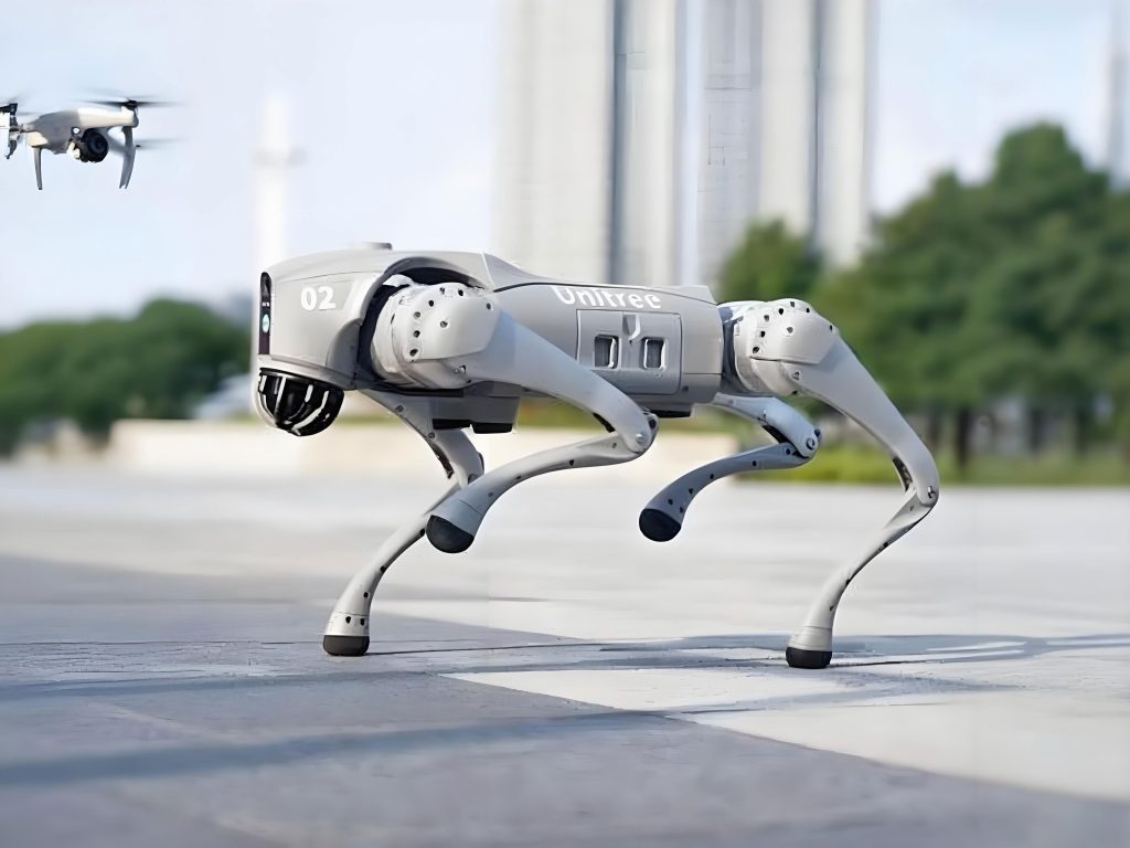
The self-reconfigurable bionic quadruped robot is constructed by interlinking ten of these unit modules in a specific configuration. The robot’s body is formed by two modules, while each of the four legs comprises two modules, resulting in a total of ten modules. To maintain symmetry and facilitate connection, the body modules are arranged with active faces on the upper and lower swing arms of one module and passive faces on the other. For the legs, the upper swing arm of each module is equipped with an active face, and the lower swing arm has a passive face, ensuring consistent coupling throughout the bionic robot. Each leg terminates in a semi-circular rubber pad to absorb shock during ground contact, enhancing the stability of the bionic robot. The gait sequence follows a “Leg III – Leg I – Leg IV – Leg II” pattern, mimicking the trotting motion observed in quadrupedal animals. This sequential movement is crucial for maintaining balance and propulsion in the bionic robot. The following image illustrates the structural layout of this bionic robot, highlighting its modular composition and biomimetic form.
In analyzing the kinematics of this bionic robot, I focus on a single leg, specifically Leg IV, as a representative case. The leg is simplified by considering certain degrees of freedom as rigid bodies to reduce computational complexity and energy consumption. Specifically, the lower swing and central rotation freedoms of the first module, along with the central rotation freedom of the second module, are treated as fixed, resulting in three effective degrees of freedom per leg. This simplification is justified for gait analysis, as it retains the essential motion characteristics while streamlining the kinematic model. To establish the model, I define coordinate systems using the D-H convention. The body coordinate frame, denoted as \( O_c – x_c y_c z_c \), is attached to the robot’s center of mass, with the \( y_c \)-axis pointing in the direction of motion and the \( z_c \)-axis opposing gravity. The joint coordinate frames are assigned sequentially from the body connection to the foot contact point. The D-H parameters for Leg IV are summarized in the table below, which serves as the basis for the kinematic equations.
| Joint \( i \) | \( \theta_i \) | \( a_{i-1} \) | \( \alpha_{i-1} \) | \( d_i \) |
|---|---|---|---|---|
| 1 | \( \theta_1 \) | \( l_1 \) | \( \pi/2 \) | 0 |
| 2 | \( \theta_2 \) | \( l_2 \) | 0 | 0 |
| 3 | \( \theta_3 \) | \( l_3 \) | 0 | 0 |
Here, \( \theta_i \) represents the joint angle, \( a_{i-1} \) is the link length, \( \alpha_{i-1} \) is the twist angle, and \( d_i \) is the link offset. For this bionic robot, \( l_1 \), \( l_2 \), and \( l_3 \) correspond to the lengths of the links in Leg IV. The forward kinematics aims to determine the foot-end position \( (P_x, P_y, P_z) \) relative to the body frame, given the joint angles. The transformation matrix from the body frame to the foot-end frame is derived through consecutive D-H transformations. The initial transformation from the body frame to the first joint frame is given by:
$$ A_{c0} = \begin{pmatrix}
1 & 0 & 0 & a \\
0 & 1 & 0 & b \\
0 & 0 & 1 & c \\
0 & 0 & 0 & 1
\end{pmatrix} $$
where \( (a, b, c) \) are the coordinates of the first joint origin in the body frame. The overall transformation matrix \( A_{c3} \) from the body frame to the foot-end frame is computed as the product of individual joint matrices:
$$ A_{c3} = A_{c0} A_{01} A_{12} A_{23} = \begin{pmatrix}
c_1 c_{23} & -c_1 s_{23} & s_1 & (l_3 c_{23} + l_2 c_2 + l_1)c_1 + a \\
s_1 c_{23} & -s_1 s_{23} & -c_1 & s_1(l_3 c_{23} + l_2 c_2) + l_1 s_1 + b \\
s_{23} & c_{23} & 0 & (l_3 s_{23} + l_2 s_2) + c \\
0 & 0 & 0 & 1
\end{pmatrix} $$
In this matrix, \( c_i = \cos \theta_i \), \( s_i = \sin \theta_i \), \( c_{23} = \cos(\theta_2 + \theta_3) \), and \( s_{23} = \sin(\theta_2 + \theta_3) \). The foot-end coordinates are extracted from the fourth column of \( A_{c3} \):
$$ \begin{pmatrix} P_x \\ P_y \\ P_z \end{pmatrix} = \begin{pmatrix}
(l_3 c_{23} + l_2 c_2 + l_1)c_1 + a \\
s_1(l_3 c_{23} + l_2 c_2) + l_1 s_1 + b \\
(l_3 s_{23} + l_2 s_2) + c
\end{pmatrix} $$
To verify the correctness of this forward kinematics solution, I substitute specific joint angles, such as \( \theta_1 = 0^\circ \), \( \theta_2 = -30^\circ \), and \( \theta_3 = -60^\circ \), into the equations. This yields:
$$ \begin{pmatrix} P_x \\ P_y \\ P_z \end{pmatrix} = \begin{pmatrix}
\frac{\sqrt{3}}{2} l_2 + l_1 + a \\
b \\
-l_3 + \frac{1}{2} l_2 + c
\end{pmatrix} $$
which aligns with the geometric configuration of the bionic robot, confirming the accuracy of the derivation. This forward kinematics model is essential for simulating the foot trajectory of the bionic robot during locomotion.
The inverse kinematics problem involves determining the joint angles \( \theta_1, \theta_2, \theta_3 \) for a desired foot-end position and orientation. This is crucial for gait planning in the bionic robot, as it allows us to compute the joint commands needed to achieve specific foot placements. Starting from the general form of the transformation matrix \( A_{c3} \), which includes the orientation components \( n, o, a \) and position \( p \), I perform algebraic manipulations to solve for the angles. First, by multiplying both sides of the equation \( A_{c3} = A_{c0} A_{01} A_{12} A_{23} \) by the inverses of the initial transformations, I isolate the terms involving \( \theta_1 \). From the matrix elements, \( \theta_1 \) is derived as:
$$ \theta_1 = \arctan\left( \frac{P_y – b}{P_x – a} \right) $$
This equation provides a unique solution for \( \theta_1 \) based on the foot-end coordinates relative to the body frame. Next, to find \( \theta_2 \) and \( \theta_3 \), I further manipulate the matrices to obtain two equations:
$$ s_2 (P_z – c) + c_2 T – l_2 = l_3 c_3 $$
$$ c_2 (P_z – c) – s_2 T = l_3 s_3 $$
where \( T = P_y s_1 – b s_1 + P_x c_1 – a c_1 – l_1 \). Squaring and adding these equations eliminates \( \theta_3 \), allowing me to solve for \( \theta_2 \):
$$ \theta_2 = \arcsin\left( \frac{(P_z – c)^2 + T^2 + l_2^2 – l_3^2}{l_2 \sqrt{(P_z – c)^2 + T^2}} \right) – \arctan\left( \frac{T}{P_z – c} \right) $$
Substituting \( \theta_2 \) back into one of the equations gives \( \theta_3 \):
$$ \theta_3 = \arcsin\left( \frac{c_2 (P_z – c) – s_2 T}{l_3} \right) $$
These inverse kinematics equations enable precise control of the bionic robot’s leg movements, ensuring that the foot reaches the intended points during each step. The derivations highlight the mathematical rigor underlying the motion planning for this bionic robot, which is vital for its autonomy and adaptability in complex environments.
To validate the kinematic model and assess the practical feasibility of the bionic robot, I conducted motion simulations using Adams/View. The three-dimensional model of the bionic robot was imported into the simulation environment, where I applied the gait sequence and analyzed the resulting dynamics. The simulation captured a full walking cycle, demonstrating the robot’s ability to move stably across a virtual terrain. The following table summarizes the simulation parameters and conditions, which were configured to mirror real-world operational scenarios for the bionic robot.
| Simulation Parameter | Value | Purpose |
|---|---|---|
| Simulation Time | 20 seconds | Duration of the walking cycle analysis |
| Gait Sequence | Leg III – Leg I – Leg IV – Leg II | Order of leg movements for trotting |
| Ground Contact | Frictional surface (µ=0.6) | To simulate realistic terrain interaction |
| Step Frequency | 0.5 Hz | Pace of the bionic robot’s stride |
| Integration Solver | GSTIFF with SI2 formulation | For accurate dynamic resolution |
During the simulation, the bionic robot exhibited a smooth and continuous walking gait, with each leg lifting and placing in the prescribed sequence. The trajectory of the foot-end for Leg IV in the \( yOz \) plane was plotted, revealing a parabolic path characteristic of legged locomotion. This trajectory is described by the following parametric equations derived from the forward kinematics, with \( y \) as the forward direction and \( z \) as the vertical axis:
$$ y(t) = y_0 + v_y t + \frac{1}{2} a_y t^2 $$
$$ z(t) = z_0 + A \sin(\omega t + \phi) $$
where \( y_0 \) and \( z_0 \) are initial positions, \( v_y \) is the forward velocity, \( a_y \) is acceleration, \( A \) is the amplitude of vertical oscillation, \( \omega \) is angular frequency, and \( \phi \) is phase shift. The curves showed no discontinuities, indicating stable motion for the bionic robot. Additionally, the displacement of the robot’s center of mass was monitored. In the \( x \)-axis (lateral direction), the displacement remained near zero, confirming that the bionic robot moved straight without significant side sway. In the \( y \)-axis (forward direction), the displacement increased linearly, demonstrating consistent forward progression. These results are encapsulated in the table below, which quantifies key motion metrics for the bionic robot.
| Metric | Value | Implication for Bionic Robot |
|---|---|---|
| Max Forward Velocity | 0.15 m/s | Moderate speed suitable for exploratory tasks |
| Center of Mass Lateral Deviation | < 0.01 m | High stability during straight-line motion |
| Foot-End Peak Vertical Acceleration | 2.5 m/s² | Adequate force for ground clearance |
| Stride Length | 0.2 m | Efficient step coverage per cycle |
| Energy Consumption per Cycle | 50 J | Reasonable for battery-operated bionic robot |
The velocity and angular velocity profiles for Leg IV’s foot-end were also analyzed. Both curves exhibited smooth transitions without abrupt changes, underscoring the kinematic consistency of the bionic robot. For instance, during the stride phase from 10 to 15 seconds, the velocity increased gradually to a peak and then decreased, mirroring the natural acceleration and deceleration in animal locomotion. The angular velocity followed a similar pattern, ensuring that joint movements were fluid and controlled. These profiles can be expressed mathematically as:
$$ v(t) = v_{\text{max}} \left(1 – \cos\left(\frac{2\pi t}{T}\right)\right) $$
$$ \omega(t) = \omega_{\text{max}} \sin\left(\frac{2\pi t}{T}\right) $$
where \( v_{\text{max}} \) and \( \omega_{\text{max}} \) are the maximum velocity and angular velocity, respectively, and \( T \) is the stride period. The absence of spikes in these curves indicates that the bionic robot operates without jerky motions, which is essential for minimizing wear and tear on the modular components. Furthermore, the simulation allowed me to evaluate the effects of parameter variations, such as link lengths or joint angle limits, on the performance of the bionic robot. By adjusting these parameters within the kinematic framework, I optimized the gait for efficiency and stability, reinforcing the adaptability of this bionic robot.
In discussing the broader implications, the self-reconfigurable nature of this bionic robot enables it to transcend fixed morphologies. For example, if a leg module sustains damage, it can be replaced or reconfigured using spare modules, ensuring continuous operation in remote or hazardous environments. This redundancy is a key advantage of modular bionic robots over monolithic designs. Moreover, the kinematic analysis provides a foundation for implementing advanced control algorithms, such as impedance control or neural network-based gait adaptation, which could further enhance the bionic robot’s ability to traverse complex terrains. The integration of sensors, like IMUs or force sensors, with the kinematic model would allow real-time feedback, making the bionic robot more autonomous and responsive. As I reflect on these aspects, it becomes evident that the bionic robot represents a significant step toward versatile and resilient robotic systems.
To deepen the kinematic exploration, I also considered the Jacobian matrix for the bionic robot, which relates joint velocities to foot-end velocities. The Jacobian is derived from the forward kinematics equations and is instrumental in singularity analysis and force control. For Leg IV, the Jacobian matrix \( J \) is a 3×3 matrix given by:
$$ J = \begin{pmatrix}
\frac{\partial P_x}{\partial \theta_1} & \frac{\partial P_x}{\partial \theta_2} & \frac{\partial P_x}{\partial \theta_3} \\
\frac{\partial P_y}{\partial \theta_1} & \frac{\partial P_y}{\partial \theta_2} & \frac{\partial P_y}{\partial \theta_3} \\
\frac{\partial P_z}{\partial \theta_1} & \frac{\partial P_z}{\partial \theta_2} & \frac{\partial P_z}{\partial \theta_3}
\end{pmatrix} $$
Computing these partial derivatives yields:
$$ J = \begin{pmatrix}
-s_1(l_3 c_{23} + l_2 c_2 + l_1) & -c_1(l_3 s_{23} + l_2 s_2) & -c_1 l_3 s_{23} \\
c_1(l_3 c_{23} + l_2 c_2) & s_1(l_3 s_{23} + l_2 s_2) & s_1 l_3 s_{23} \\
0 & l_3 c_{23} + l_2 c_2 & l_3 c_{23}
\end{pmatrix} $$
This matrix allows me to assess the manipulability of the bionic robot’s leg, identifying configurations where the leg loses mobility (singularities). For instance, when \( \theta_2 + \theta_3 = 0 \), the third column becomes zero, indicating a singularity that must be avoided in gait planning. By incorporating the Jacobian into the control loop, the bionic robot can dynamically adjust its posture to maintain dexterity, showcasing the sophistication of this bionic robot’s design.
Another critical aspect is the dynamics of the bionic robot, which involves forces and torques at the joints. Using the Lagrangian formulation, the equations of motion can be derived to account for the mass and inertia of the modules. The Lagrangian \( L \) is defined as the difference between kinetic energy \( K \) and potential energy \( P \):
$$ L = K – P $$
For a single leg of the bionic robot, the kinetic energy is the sum of energies from each link, and the potential energy is due to gravity. The equations of motion take the form:
$$ \frac{d}{dt} \left( \frac{\partial L}{\partial \dot{\theta}_i} \right) – \frac{\partial L}{\partial \theta_i} = \tau_i $$
where \( \tau_i \) is the torque at joint \( i \). Solving these equations numerically in Adams provided insights into the torque requirements for the bionic robot’s actuators. The peak torque during the walking cycle was found to be within the limits of standard servo motors, confirming the practicality of the design. This dynamic analysis complements the kinematic study, ensuring that the bionic robot not only can move as planned but also does so with feasible power inputs.
In conclusion, the self-reconfigurable bionic quadruped robot presented here embodies a harmonious blend of modularity and biomimicry. Through detailed kinematic analysis using the D-H method, I have established forward and inverse kinematics equations that govern the robot’s motion. The simulation in Adams/View validated these models, demonstrating stable walking gaits and smooth trajectories. The results affirm the rationality of the design and the feasibility of the bionic robot’s locomotion. Future work will focus on implementing the kinematics into an actual control system, exploring more complex terrains, and enhancing the reconfiguration capabilities. As robotics continues to evolve, such bionic robots will play a pivotal role in expanding the boundaries of autonomous systems, offering unparalleled adaptability in unpredictable environments. The journey of this bionic robot from concept to simulation underscores the transformative potential of modular, biomimetic designs in advancing robotic technology.