
In the context of modern intelligent manufacturing and service robotics, the embodied robot concept has shifted from isolated manipulators to integrated mobile manipulation platforms. A wheeled humanoid robot, as a typical embodiment of this concept, combines the dexterity of multi-degree-of-freedom (DOF) arms with the mobility of an automated guided vehicle. In this thesis, I focus on the design and implementation of a whole-body motion control system for such an embodied robot. The core challenge lies in the high-dimensional, strongly coupled kinematics and dynamics of the system. Instead of treating the mobile base and the upper-body manipulator as separate entities, I investigate coordinated control strategies that exploit the redundancy of the entire kinematic chain. This allows the robot to execute tasks efficiently while respecting safety constraints such as joint limits, velocity bounds, self-collision avoidance, and tip-over prevention.
The main contributions of this work are threefold. First, I establish a complete hardware and software architecture for a self-developed wheeled humanoid robot, covering mechanical design, actuator selection, sensor integration, communication schemes, and ROS2-based software stacks. Second, I derive a whole-body kinematic model and propose a task-space control framework using Jacobian pseudo-inverse and quadratic programming, augmented with control barrier functions to guarantee safety. Third, I develop a model predictive control (MPC) scheme based on the sequential linear quadratic (SLQ) algorithm, which incorporates complex constraints in a unified optimization formulation. Both simulation and physical experiments demonstrate the effectiveness and real-time feasibility of the proposed methods. Throughout this thesis, the term embodied robot highlights the closed-loop interaction between morphological structure, actuation, sensing, and computation.
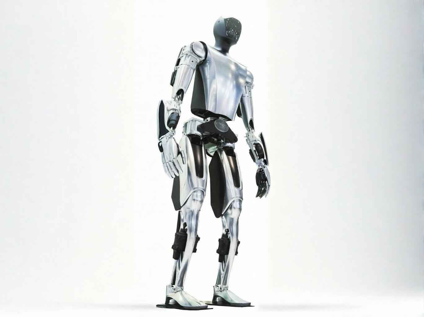
1. System Architecture and Hardware Design
I started the design by specifying the performance requirements according to the intended indoor logistics and service scenarios. The wheeled humanoid robot must be able to navigate in narrow spaces, reach objects on shelves at various heights, and manipulate them with sufficient precision. Table 1 summarizes the main performance indicators that guide the mechanical and electrical design.
| Property | Value |
|---|---|
| Height | 1700 mm |
| Mass | 80 kg |
| Protection class | IP21 (indoor) |
| Active DOF | 32 |
| Maximum linear velocity | 2 m/s |
| Arm DOF (single) | 6 |
| Arm reach | 600 mm |
| Payload per arm | ≥3 kg (dual arm ≥6 kg) |
| Repeatability | ±0.2 mm |
| Dexterous hand DOF | 6 active per hand |
| AI computational power | ≥100 TOPS |
| Battery capacity | 60 Ah, 48 V |
| Estimated endurance | ≥4 h |
The robot body consists of a differential-drive mobile base, a 3-DOF leg, a 1-DOF torso, two 6-DOF arms, two 6-DOF dexterous hands, and a 2-DOF head. The active DOF distribution is given in Table 2. The mobile base uses two servo-driven wheels in the front and two passive casters in the rear, providing stable support while allowing agile turning. The leg joints are collinear in the sagittal plane, enabling the robot to adjust its overall height and center of mass. The torso adds a yaw rotation to expand the workspace of the upper body.
| Part | Number of DOF |
|---|---|
| Mobile base | 2 |
| Leg | 3 |
| Torso | 1 |
| Head | 2 |
| Arm (each) | 6 |
| Hand (each) | 6 |
| Total | 32 |
1.1 Kinematic Modeling of the Mobile Base
For a differential-drive mobile base, I define the world frame \(\{W\}\) and the base frame \(\{B\}\). The pose of the base is described by \( (x_b, y_b, \phi_b) \). The linear velocity of the base along its heading is \(v_b\), and the angular velocity is \(\omega_b\). The left and right wheel angular velocities are \(\dot{\theta}_L\) and \(\dot{\theta}_R\), respectively. The wheel radius is \(r\), and the distance between the two drive wheels is \(d\). The forward kinematics of the base can be written as:
\[
\begin{bmatrix}
\dot{x}_b \\ \dot{y}_b \\ \dot{\phi}_b
\end{bmatrix}
=
\begin{bmatrix}
\frac{r\cos\phi_b}{2} & \frac{r\cos\phi_b}{2} \\
\frac{r\sin\phi_b}{2} & \frac{r\sin\phi_b}{2} \\
\frac{r}{d} & -\frac{r}{d}
\end{bmatrix}
\begin{bmatrix}
\dot{\theta}_R \\ \dot{\theta}_L
\end{bmatrix}.
\]
This equation maps the actuator rates to the base velocity in the world frame. For the whole-body model, I treat the base as a virtual prismatic-revolute joint that can rotate and translate in the plane, which simplifies the derivation of the full Jacobian.
1.2 Kinematic Modeling of the Arm
Each arm is modeled as a 6-DOF serial manipulator using standard Denavit–Hartenberg (D-H) parameters. The D-H table for the right arm is shown in Table 3. The transformation from the shoulder base frame to the end-effector frame is obtained by consecutive matrix multiplications.
| Joint \(i\) | \(\theta_i\) | \(d_i\) (m) | \(a_i\) (m) | \(\alpha_i\) |
|---|---|---|---|---|
| 1 | \(\theta_{shoulder\_y}\) | 0 | 0.15 | 0 |
| 2 | \(\theta_{shoulder\_x} + \pi/2\) | 0.20 | 0.04 | \(-\pi/2\) |
| 3 | \(\theta_{elbow\_z} – \pi/2\) | 0 | 0.15 | \(-\pi/2\) |
| 4 | \(\theta_{elbow\_y} – \pi/2\) | 0 | 0.15 | \(-\pi/2\) |
| 5 | \(\theta_{wrist\_x} + \pi/2\) | 0 | 0.12 | \(\pi/2\) |
| 6 | \(\theta_{wrist\_z}\) | 0 | 0.10 | 0 |
The forward kinematics of the entire upper body (leg + torso + arm) can be expressed as a single homogeneous transformation matrix \( \mathbf{T}^e_a(\mathbf{q}_s) \), where \(\mathbf{q}_s\) is the vector of joint angles of the serial chain starting at the ankle and ending at the end-effector.
2. Hardware and Communication Design
I adopted a dual-controller architecture to balance real-time motion planning and AI-based perception. A Raspberry Pi 5 handles the upper body control, while an NVIDIA Jetson Orin Nano handles the lower body and navigation tasks. The two controllers communicate via a wired Ethernet link, which provides high bandwidth and low latency for ROS2 communication. Table 4 lists the key hardware components selected for the embodied robot.
| Component | Model / Specification |
|---|---|
| Main controller (upper body) | Raspberry Pi 5, quad-core Cortex-A76, 8 GB RAM |
| Main controller (lower body) | NVIDIA Jetson Orin Nano, 6-core Cortex-A78AE, 8 GB LPDDR5 |
| Joint actuator | Integrated joint module with harmonic drive, dual encoder, torque sensor |
| Drive wheel | Integrated servo wheel, rated torque 21 N·m, CANopen |
| Depth camera | Intel RealSense D435i, 1280×720 depth, 90 fps |
| LiDAR | Unitree L1 4D LiDAR, 360°×90°, range 30 m |
| IMU | Wheeltec N100, 9-axis, 400 Hz output |
| Power | 48 V, 60 Ah lithium battery |
The electrical power distribution is shown in Table 5. The 48 V battery directly powers the joint modules and the servo wheels. Step-down converters generate 24 V and 19 V supplies for the controllers, sensors, and human-machine interface modules.
| Voltage rail | Consumers |
|---|---|
| 48 V | Joint modules, servo wheels |
| 24 V | Head, hands, light indicators |
| 19 V | Raspberry Pi, Jetson Orin Nano |
| 5 V / 3.3 V | Sensors via USB or GPIO |
For communication, I used CAN bus for all actuators. The Raspberry Pi is extended with two CAN adapters, and the Jetson Orin Nano has an onboard CAN controller. A STM32 microcontroller is used as a communication bridge for additional motor groups, providing two extra CAN channels. Sensors communicate via USB/UART. The overall communication topology ensures that all joint commands and state feedback can be exchanged at frequencies up to 1 kHz.
3. Software System Design
The software stack follows a layered, modular architecture built on ROS2. At the lowest level, the hardware driver layer uses ros2_control to abstract all actuators and sensors. I implemented a ros2_canopen based driver for the joint modules, which automatically configures PDO/SDO mappings and synchronizes the bus. The controller layer integrates standard controllers such as joint trajectory controllers, velocity controllers, and differential drive controllers. On top of that, MoveIt2 handles motion planning for the arms and upper body, while Nav2 handles global and local navigation of the mobile base.
The entire software pipeline is designed as a set of ROS2 nodes. The main nodes include:
- Robot state publisher: broadcasts the URDF and joint transforms.
- Joint state broadcaster: publishes measured joint positions, velocities, and torques.
- MoveIt2 move_group: provides inverse kinematics, collision checking, and trajectory planning.
- Nav2 server: handles path planning and base velocity commands.
- Whole-body controller: executes the proposed QP or MPC algorithms and outputs joint velocity commands.
I also designed a teleoperation subsystem using a gamepad. The moveit_servo package is used to send Cartesian velocity commands or joint jog commands. The mapping of the gamepad buttons to the robot motions is defined in Table 6.
| Gamepad input | Robot command |
|---|---|
| Left joystick Y-axis | Base linear velocity |
| Left joystick X-axis | Base angular velocity |
| Right joystick | End-effector Cartesian velocity |
| Button A + left joystick | Head pan/tilt |
| Button B + right joystick | Arm joint jog |
| Button X | Gripper open/close |
The autonomous docking and charging system is based on opennav_docking. A QR tag on the charging station is detected by the head-mounted camera, and a visual servoing loop refines the alignment. Once the robot reaches the dock, it verifies the charging current and enters a low-power state.
4. Whole-Body Kinematics and Task Jacobian
For the whole-body motion control, I consider the robot as a mobile manipulator consisting of a mobile base plus a serial chain formed by the leg, torso, and right arm. The generalized coordinate vector is \(\mathbf{q} = [\mathbf{q}_b^\top, \mathbf{q}_s^\top]^\top \in \mathbb{R}^{n}\), where \(\mathbf{q}_b \in \mathbb{R}^2\) represents the virtual base coordinates (position along the heading direction and rotation angle), and \(\mathbf{q}_s \in \mathbb{R}^{m}\) represents the joint angles of the serial chain. The forward kinematics of the end-effector is given by:
\[
\mathbf{T}^w_e(\mathbf{q}) = \mathbf{T}^w_b(\mathbf{q}_b) \mathbf{T}^b_a \mathbf{T}^a_e(\mathbf{q}_s),
\]
where \(\mathbf{T}^b_a\) is a constant transformation from the base frame to the ankle frame. By differentiating this expression with respect to time, I obtain the differential kinematic relation:
\[
\mathbf{v}_e = \mathbf{J}_e(\mathbf{q}) \dot{\mathbf{q}},
\]
where \(\mathbf{v}_e \in \mathbb{R}^6\) is the end-effector spatial twist in the world frame, and \(\mathbf{J}_e \in \mathbb{R}^{6 \times n}\) is the whole-body Jacobian matrix. This Jacobian is computed efficiently using the Pinocchio library, which also provides analytical derivatives.
4.1 Task Jacobian and Pseudo-Inverse Control
I first explored a pseudo-inverse based controller for whole-body redundancy resolution. For a position task defined by the residual \(\mathbf{e}_p = \mathbf{p}_e – \mathbf{p}_e^*\), I choose the joint velocity as:
\[
\dot{\mathbf{q}} = \mathbf{J}_p^\dagger(\mathbf{q}) ( -K_p \mathbf{e}_p ),
\]
where \(\mathbf{J}_p\) is the position Jacobian and \(\mathbf{J}_p^\dagger\) denotes the Moore–Penrose pseudoinverse. For tasks involving orientation, I express the orientation error in the Lie algebra of SO(3). The relative twist error is given by:
\[
\mathbf{e}_o = \log\!\left( \mathbf{R}_e^\top \mathbf{R}_e^* \right)^\vee.
\]
Then the task Jacobian in the local frame is used to map joint velocities to the angular velocity error. This approach is straightforward but suffers from the inability to incorporate inequality constraints. Joint limits, velocity limits, and self-collision avoidance are easily violated during aggressive motions.
4.2 Quadratic Programming with Control Barrier Functions
To handle constraints, I formulated the whole-body inverse kinematics as a Quadratic Programming (QP) problem. The optimization variable is the joint velocity \(\dot{\mathbf{q}}\). The objective is the weighted sum of task errors, and the constraints include joint velocity bounds and joint position limits. The QP is written as:
\[
\min_{\dot{\mathbf{q}}} \sum_i w_i \left\| \mathbf{J}_i \dot{\mathbf{q}} – \mathbf{v}_i^{ref} \right\|^2 + \lambda \| \dot{\mathbf{q}} \|^2,
\]
\[
\text{subject to } \dot{\mathbf{q}}^- \le \dot{\mathbf{q}} \le \dot{\mathbf{q}}^+,
\]
\[
K_{lim} \frac{\mathbf{q}^- – \mathbf{q}}{\Delta t} \le \dot{\mathbf{q}} \le K_{lim} \frac{\mathbf{q}^+ – \mathbf{q}}{\Delta t}.
\]
The parameter \(K_{lim}\) controls how aggressively the joint limits are enforced. I also added acceleration limits to smooth the solution:
\[
\ddot{\mathbf{q}}^- \le \frac{\dot{\mathbf{q}}(k) – \dot{\mathbf{q}}(k-1)}{\Delta t} \le \ddot{\mathbf{q}}^+.
\]
Self-collision avoidance was realized by incorporating Control Barrier Functions (CBF). For the \(j\)-th collision pair, I define a safety function \(h_j(\mathbf{q})\) representing the signed distance between the two collision bodies minus a safety margin. The CBF condition is:
\[
\frac{\partial h_j}{\partial \mathbf{q}} \dot{\mathbf{q}} + \alpha_j h_j(\mathbf{q}) \ge 0.
\]
This inequality is linear in \(\dot{\mathbf{q}}\) and thus can be appended to the QP. I selected several critical collision pairs on the embodied robot, such as the forearm against the torso, and the upper arm against the head. This CBF-QP controller improved the success rate of reaching random poses compared to the pure pseudo-inverse method.
5. Model Predictive Control for Whole-Body Motion
Although the QP approach can respect convex constraints, it is difficult to incorporate future predictions and more complex constraints such as the robot center-of-mass (CoM) position or non-convex obstacles. Model predictive control provides a principled way to handle these issues. I adopted the SLQ-MPC algorithm from the OCS2 toolbox, which solves the optimal control problem with a sequential linear quadratic approach. The algorithm iteratively linearizes the system dynamics around the current nominal trajectory and solves a constrained time-varying LQR problem.
5.1 Problem Formulation
The state vector is \(\mathbf{x} = [\mathbf{p}_b^\top, \boldsymbol{\phi}_b, \mathbf{q}_s^\top]^\top\), where \(\mathbf{p}_b\) and \(\boldsymbol{\phi}_b\) denote the base position and heading, respectively. The control input is \(\mathbf{u} = [v_b, \omega_b, \dot{\mathbf{q}}_s^\top]^\top\). The system dynamics is simply the kinematic evolution:
\[
\dot{\mathbf{x}} = \mathbf{f}(\mathbf{x}, \mathbf{u}),
\]
which is derived from the forward kinematics and the base model. The cost function is defined as:
\[
J = \int_0^{T} \left( \sum_i \left\| \mathbf{e}_{p,i}(t) \right\|^2_{\mathbf{Q}_p} + \left\| \mathbf{e}_{o,i}(t) \right\|^2_{\mathbf{Q}_o} + \mathbf{u}(t)^\top \mathbf{R} \mathbf{u}(t) + \sum_j B_j(\mathbf{x}(t), \mathbf{u}(t)) \right) dt,
\]
where \(\mathbf{e}_{p,i}\) and \(\mathbf{e}_{o,i}\) are the position and orientation errors of the \(i\)-th end-effector, and \(B_j\) are relaxed barrier functions representing the inequality constraints.
5.2 Constraints as Relaxed Barrier Functions
I used a smooth relaxed barrier function to penalize constraint violations without causing numerical ill-conditioning. The function is:
\[
B(z) = \begin{cases}
-\mu \ln(z), & z > \delta, \\
\mu \beta(z), & z \le \delta,
\end{cases}
\]
where \(z\) denotes the difference between the constrained quantity and its limit, \(\mu\) is a weight, and \(\beta(z)\) is a quadratic smoothing function. Table 7 lists the constraints implemented through these barrier terms.
| Constraint type | Expression | Purpose |
|---|---|---|
| Joint position limits | \(q_i^{\min} \le q_i \le q_i^{\max}\) | Respect mechanical stroke |
| Control input limits | \(v^{\min} \le v_b \le v^{\max}\), \(\omega^{\min} \le \omega_b \le \omega^{\max}\) | Respect actuator capabilities |
| Joint speed limits | \(\dot{q}_i^{\min} \le \dot{q}_i \le \dot{q}_i^{\max}\) | Prevent excessive speed |
| Self-collision avoidance | \(d_j(\mathbf{x}) – \epsilon_j \ge 0\) | Prevent robot self-contact |
| Anti-tip-over | \(r_{CoG} \le r_{support}\) | Maintain CoM inside support polygon |
5.3 Simplification of the Anti-Tip-over Constraint
Computing the center-of-mass position in every MPC iteration adds computational burden. To improve real-time performance, I converted the anti-tip-over constraint into a joint position constraint on the leg. By analyzing the extreme posture where the robot carries the maximum payload in the horizontal direction, I derived an admissible range for the leg joint angles that guarantees the CoM remains inside the support circle. This simplification is valid because the SLQ-MPC already limits base accelerations and joint velocities to moderate values, so dynamic effects on the CoM are negligible. The resulting controller becomes more computationally efficient while still avoiding tip-over.
5.4 Simulation and Experimental Results
I validated the MPC controller in both simulation and on the physical robot. The task was to move the end-effector from its initial configuration to a target pose \(\mathbf{p}^* = [2.0, 0, 0.8]^\top\) meters and orientation quaternion \(\mathbf{q}^* = [0.707, 0, 0.707, 0]\). The simulation parameters are summarized in Table 8.
| Parameter | Value |
|---|---|
| MPC horizon \(T\) | 1.0 s |
| Sampling time \(\Delta t\) | 20 ms |
| Base velocity limits | ±0.5 m/s |
| Base angular velocity limits | ±0.5 rad/s |
| Joint velocity limits | ±0.5 rad/s |
| Input weight \(\mathbf{R}_{base}\) | \(0.05 \mathbf{I}_{2}\) |
| Input weight \(\mathbf{R}_{arm}\) | \(0.01 \mathbf{I}_{7}\) |
| Position error weight \(\mathbf{Q}_p\) | \(10 \mathbf{I}_{3}\) |
| Orientation error weight \(\mathbf{Q}_o\) | \(5 \mathbf{I}_{3}\) |
The position error and orientation error are shown in Figure 1 (not inserted due to layout). The errors converge to zero in about 20 seconds. The base linear velocity and angular velocity remain within the prescribed limits. The joint positions also stay inside the allowable ranges. The cost function decreases rapidly and reaches its minimum after about 25 seconds, indicating a fast convergence of the SLQ-MPC algorithm.
I also performed a comparative experiment with and without the anti-tip-over constraint. Without the constraint, the CoM trajectory eventually leaves the support polygon, leading to tip-over. With the constraint, the CoM remains always inside the support circle. This verifies the effectiveness of the proposed anti-tip-over simplification.
To statistically evaluate the control method, I sampled 50 random target poses in the workspace ahead of the robot. The success rate reached 96%. The average task completion time was 14.2 seconds, and the average path length of the end-effector was 1.32 meters. These results demonstrate that the MPC-based whole-body controller is both efficient and reliable for the considered embodied robot platform.
6. Conclusion and Future Work
In this thesis, I presented a comprehensive study on the whole-body motion control of a wheeled humanoid robot. I designed the hardware architecture, implemented the ROS2-based software stack, and developed two control frameworks: one based on quadratic programming with control barrier functions, and another based on model predictive control with a sequential linear quadratic solver. Both methods were validated through simulations and physical experiments, showing that the embodied robot can execute tasks with high precision while satisfying safety constraints.
The key findings are summarized below:
- The pseudo-inverse method is simple but often violates constraints during large motions.
- The QP-CBF approach effectively handles joint limits, speed limits, and self-collision avoidance, but it is less suitable for long-horizon tasks or complex constraints involving the center of mass.
- The SLQ-MPC method offers superior performance in terms of constraint satisfaction and predictive planning, at the cost of increased computational complexity.
- The conversion of the anti-tip-over constraint into joint position limits greatly improves the real-time performance of the MPC controller.
Future work will focus on incorporating visual feedback directly into the MPC cost function to enable visual servoing for object grasping. I also plan to extend the framework to bimanual manipulation, where both arms and the mobile base must be coordinated simultaneously. The robustness of the controller under external disturbances will be investigated further, and the algorithms will be deployed on more complex embodied robot platforms.