
The pursuit of high precision, compactness, and reliability in modern robotics has placed stringent demands on joint drive mechanisms. Among these, the RV reducer stands out due to its exceptional characteristics: a large transmission ratio, high torsional stiffness, substantial load capacity, and excellent positioning accuracy. Consequently, the RV reducer has become a critical and widely adopted component in industrial robotic joints. Despite its advantages, the complex vibration and noise signatures of the RV reducer present significant challenges for its design and application. A fundamental step in vibration analysis and noise reduction is the accurate identification of all potential excitation sources, which are intrinsically linked to the operating frequencies of its numerous moving parts. Given the RV reducer‘s intricate two-stage, closed, and statically indeterminate structure, calculating these frequencies is non-trivial. This work aims to establish a comprehensive, generalized theoretical framework for computing all significant operating frequencies within an RV reducer, encompassing both transmission components and rolling bearing elements, and to validate this framework through dynamic simulation.
Transmission Principle and Operational Modes of the RV Reducer
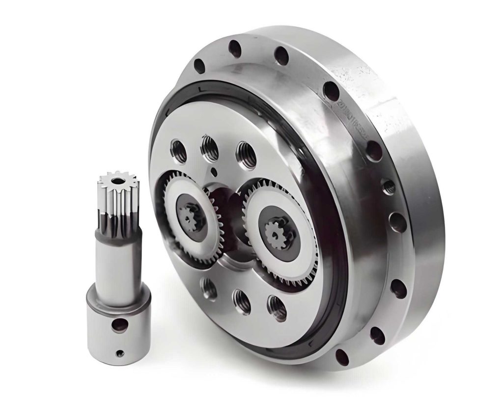
The RV reducer is a compound planetary transmission system that ingeniously combines a first-stage involute planetary gear train with a second-stage cycloidal-pin gear planetary mechanism. Its compact and rigid structure typically employs a central support disc configuration. The power flow and component interaction can be understood through two primary operational modes, dictated by which member is held stationary: the support disc or the pin wheel.
In the first mode, with the Support Disc Fixed, the input rotation is applied to the sun gear. This drives the planetary gears, which are rigidly connected to the crankshafts. Since the planetary gears mesh with the fixed sun gear, they, and consequently the crankshafts, undergo pure rotation (autorotation) without revolution around the sun gear center. The eccentric portion of each crankshaft, via a crank bearing (often a needle roller bearing), imparts a pure revolutionary motion to the cycloidal disc around the center of the pin wheel. The meshing between the cycloidal disc and the fixed pin wheel forces the cycloidal disc to have zero autorotation. This revolutionary motion is directly transferred to the output member, which is the pin wheel (or the housing connected to it).
The second mode, with the Pin Wheel Fixed, is the more common configuration for robotic applications. Here, the input is still applied to the sun gear. The planetary gears, meshing with the sun gear, now experience both autorotation and revolution (carrier rotation). The crankshafts, fixed to the planets, inherit this compound motion. The crank bearings transmit this motion to the cycloidal discs, causing them to revolve around the fixed pin wheel center. The meshing with the fixed pin wheel now induces an autorotation of the cycloidal discs. This autorotation is opposite in direction to the revolution. The autorotation of the cycloidal disc is transmitted back through the crankshafts to the carrier (support disc), which becomes the output member. This dual-path load sharing contributes to the high stiffness and load capacity of the RV reducer.
Theoretical Derivation of Operating Frequencies
To systematically analyze the vibration spectrum, we must calculate the rotational frequencies of all moving parts and the meshing frequencies. We define the following rotational speeds (rpm): $n_1$ for the sun gear, $n_2$ for the crankshaft autorotation, $n_3$ for the crankshaft revolution (carrier speed), $n_4$ for the cycloidal disc autorotation, $n_5$ for the cycloidal disc revolution, $n_6$ for the pin wheel, and $n_7$ for the support disc (carrier). The corresponding frequencies in Hertz are $f_i = n_i / 60$.
Frequencies of Transmission Components
The calculations leverage the fundamental principle of planetary gear kinematics, often using the “fixed carrier” or “inversion” method. Let $z_1$, $z_2$, $z_3$, and $z_4$ represent the number of teeth for the sun gear, planetary gear, cycloidal disc, and pin wheel, respectively.
1. Support Disc Fixed Mode ($n_3 = n_4 = n_7 = 0$):
In this mode, the crankshaft revolution, cycloid autorotation, and support disc speeds are zero. The crankshaft autorotation equals the cycloid revolution ($n_2 = n_5$). Applying the inversion method to the first-stage planetary train (with carrier $n_3=0$) and relating the second-stage motion yields:
$$n_2 = n_5 = -\frac{z_1}{z_2} n_1$$
$$n_6 = -\frac{(z_4 – z_3) z_1}{z_2 z_4} n_1$$
The negative sign indicates direction opposite to the sun gear input.
2. Pin Wheel Fixed Mode ($n_6 = 0$):
In this standard mode, the crankshaft revolution, cycloid autorotation, and support disc (output) speeds are equal ($n_3 = n_4 = n_7$). The crankshaft autorotation equals the cycloid revolution ($n_2 = n_5$). The kinematic equations are derived by considering both planetary stages simultaneously:
$$n_2 = n_5 = \frac{z_1 z_4}{(z_3 – z_4) (z_1 + z_2 z_4)} n_1$$
$$n_3 = n_4 = n_7 = \frac{z_1}{z_1 + z_2 z_4} n_1$$
From these speed equations, the rotational frequencies $f_i$ and the gear meshing frequencies are readily obtained. The meshing frequency for the first stage ($f_{1c}$) is the absolute relative frequency between the sun and planet gears. For the second stage ($f_{2c}$), it is the absolute relative frequency between the cycloidal disc and the pin wheel. The results are consolidated in Table 1.
| Component / Frequency | Support Disc Fixed | Pin Wheel Fixed |
|---|---|---|
| Sun Gear Rotation ($f_1$) | $f_1 = n_1/60$ | $f_1 = n_1/60$ |
| Crankshaft Autorotation ($f_2$) | $f_2 = -\frac{z_1}{z_2} f_1$ | $f_2 = \frac{z_1 z_4}{(z_3 – z_4) (z_1 + z_2 z_4)} f_1$ |
| Crankshaft Revolution ($f_3$) | $f_3 = 0$ | $f_3 = \frac{z_1}{z_1 + z_2 z_4} f_1$ |
| Cycloid Disc Autorotation ($f_4$) | $f_4 = 0$ | $f_4 = \frac{z_1}{z_1 + z_2 z_4} f_1$ |
| Cycloid Disc Revolution ($f_5$) | $f_5 = -\frac{z_1}{z_2} f_1$ | $f_5 = \frac{z_1 z_4}{(z_3 – z_4) (z_1 + z_2 z_4)} f_1$ |
| Pin Wheel Rotation ($f_6$) | $f_6 = -\frac{(z_4 – z_3) z_1}{z_2 z_4} f_1$ | $f_6 = 0$ |
| Support Disc Rotation ($f_7$) | $f_7 = 0$ | $f_7 = \frac{z_1}{z_1 + z_2 z_4} f_1$ |
| 1st Stage Mesh Frequency ($f_{1c}$) | $f_{1c} = z_1 f_1$ | $f_{1c} = \frac{z_1 z_2 z_4}{z_1 + z_2 z_4} f_1$ |
| 2nd Stage Mesh Frequency ($f_{2c}$) | $f_{2c} = \frac{z_1 z_3}{z_2} f_1$ | $f_{2c} = \frac{z_1 z_3 z_4}{z_1 + z_2 z_4} f_1$ |
Frequencies of Rolling Bearing Components
The RV reducer contains several critical bearing sets: the crankshaft support bearings, the crank bearings (connecting the crankshaft eccentric to the cycloidal disc), and the main output bearings. Each bearing’s inner race, outer race, rolling elements, and cage contribute characteristic frequencies to the vibration spectrum. The calculation is based on the assumption of pure rolling between rolling elements and raceways, neglecting slippage and elastic deformation. Key bearing geometric parameters are defined in Table 2.
| Parameter | Crank Support Bearing | Crank Bearing | Main Bearing |
|---|---|---|---|
| Pitch Diameter | $D_1$ | $D_2$ | $D_3$ |
| Roller Diameter | $d_1$ | $d_2$ | $d_3$ |
| Inner Raceway Contact Radius | $r_{11}$ | $r_{21}$ | $r_{31}$ |
| Outer Raceway Contact Radius | $r_{12}$ | $r_{22}$ | $r_{32}$ |
| Contact Angle | $\alpha_1$ | $\alpha_2$ | $\alpha_3$ |
| Number of Rollers | $Z_1$ | $Z_2$ | $Z_3$ |
Where $r_{i1} \approx (D_i – d_i \cos\alpha_i)/2$ and $r_{i2} \approx (D_i + d_i \cos\alpha_i)/2$ for $i=1,2,3$.
The fundamental kinematic relationship states that the linear velocity at the cage (rolling element center) is the average of the inner and outer raceway contact velocities: $v_c = \frac{1}{2}(v_i + v_o) = \pi f_c D$. From this, the cage rotation frequency $f_c$ (which is the roller pass frequency) can be derived relative to the inner race frequency $f_i$ and outer race frequency $f_o$. The roller autorotation frequency $f_{bc}$ is found by considering the pure rolling condition between the roller and a raceway in the cage reference frame. The frequencies for a single roller passing over a defect on the outer race ($f_{oc}$) and inner race ($f_{ic}$) are derived from the relative motion between the cage and the races. The complete set of formulas for both operational modes of the RV reducer is presented in Table 3. Note that for typical RV reducer designs, the crank support bearing is often a deep groove ball bearing ($\alpha_1 \approx 0^\circ$), the crank bearing is a needle roller bearing ($\alpha_2 \approx 0^\circ$), and the main bearing is an angular contact ball bearing ($\alpha_3 \approx 30^\circ-40^\circ$).
| Bearing | Frequency | Support Disc Fixed | Pin Wheel Fixed |
|---|---|---|---|
| Crank Support Bearing | Cage ($f_{c1}$) | $\frac{1}{2}f_2\left(1-\frac{d_1}{D_1}\cos\alpha_1\right)$ | $\frac{1}{2}\left[\left(1-\gamma_1\right)(f_2+f_3) + \left(1+\gamma_1\right)f_7\right]$ $\gamma_1=\frac{d_1}{D_1}\cos\alpha_1$ |
| Outer Race Defect ($f_{oc1}$) | $-\frac{1}{2}f_2\left(1-\gamma_1\right)$ | $-\frac{1}{2}f_2\left(1-\gamma_1\right)$ | |
| Inner Race Defect ($f_{ic1}$) | $\frac{1}{2}f_2\left(1+\gamma_1\right)$ | $\frac{1}{2}f_2\left(1+\gamma_1\right)$ | |
| Roller Spin ($f_{bc1}$) | $\frac{D_1 f_2}{2d_1}\left[1-\gamma_1^2\right]$ | $\frac{D_1 f_2}{2d_1}\left[1-\gamma_1^2\right]$ | |
| Crank Bearing | Cage ($f_{c2}$) | $\frac{1}{2}f_2\left(1-\frac{d_2}{D_2}\cos\alpha_2\right)$ | $\frac{1}{2}\left[\left(1-\gamma_2\right)(f_2+f_3) + \left(1+\gamma_2\right)f_7\right]$ $\gamma_2=\frac{d_2}{D_2}\cos\alpha_2$ |
| Outer Race Defect ($f_{oc2}$) | $-\frac{1}{2}f_2\left(1-\gamma_2\right)$ | $-\frac{1}{2}f_2\left(1-\gamma_2\right)$ | |
| Inner Race Defect ($f_{ic2}$) | $\frac{1}{2}f_2\left(1+\gamma_2\right)$ | $\frac{1}{2}f_2\left(1+\gamma_2\right)$ | |
| Roller Spin ($f_{bc2}$) | $\frac{D_2 f_2}{2d_2}\left[1-\gamma_2^2\right]$ | $\frac{D_2 f_2}{2d_2}\left[1-\gamma_2^2\right]$ | |
| Main Bearing | Cage ($f_{c3}$) | $\frac{1}{2}f_6\left(1+\frac{d_3}{D_3}\cos\alpha_3\right)$ | $\frac{1}{2}f_7\left(1-\gamma_3\right)$ $\gamma_3=\frac{d_3}{D_3}\cos\alpha_3$ |
| Outer Race Defect ($f_{oc3}$) | $\frac{1}{2}f_6\left(1-\gamma_3\right)$ | $-\frac{1}{2}f_7\left(1-\gamma_3\right)$ | |
| Inner Race Defect ($f_{ic3}$) | $-\frac{1}{2}f_6\left(1+\gamma_3\right)$ | $\frac{1}{2}f_7\left(1+\gamma_3\right)$ | |
| Roller Spin ($f_{bc3}$) | $-\frac{D_3 f_6}{2d_3}\left[1-\gamma_3^2\right]$ | $\frac{D_3 f_7}{2d_3}\left[1-\gamma_3^2\right]$ |
Numerical Example and ADAMS Simulation Validation
To demonstrate the application of the theoretical formulas and verify their accuracy, a specific RV reducer model, the RV-40E, is analyzed. The input speed is set at $n_1 = 1500$ rpm ($f_1=25$ Hz). The key parameters are as follows:
- Gearing: $z_1=16$, $z_2=32$, $z_3=39$, $z_4=40$.
- Crank Support Bearing (Deep Groove Ball): $D_1=25$ mm, $d_1=6.38$ mm, $\alpha_1=0^\circ$, $Z_1=10$.
- Crank Bearing (Needle Roller): $D_2=27$ mm, $d_2=2$ mm, $\alpha_2=0^\circ$, $Z_2=24$.
- Main Bearing (Angular Contact Ball): $D_3=130$ mm, $d_3=8$ mm, $\alpha_3=34^\circ$, $Z_3=36$.
Substituting these parameters into the formulas from Tables 1 and 3 yields the theoretical operating frequencies. To validate these results, a dynamic simulation was performed using ADAMS software. A simplified three-dimensional model of the RV reducer was created, focusing on kinematic constraints. Necessary simplifications included modeling a single cycloidal disc, merging non-critical components, and defining appropriate joints and contacts (revolute joints, fixed joints, and 3D contact forces for gear meshes and bearing interactions). The input speed was applied to the sun gear as a step function. Post-simulation, the angular velocity of each component was extracted from the software’s post-processor. For components with compound motion (e.g., crankshaft in pin-wheel-fixed mode), the absolute angular velocity from ADAMS was decomposed into autorotation and revolution components based on known kinematic relationships. The simulation results, converted to frequencies (Hz), are compared against the theoretical predictions in Table 4. The percentage error is calculated based on the absolute values: $\text{Error} = \frac{|\text{Theoretical}| – |\text{Simulation}|}{|\text{Simulation}|} \times 100\%$.
| Frequency (Hz) | Support Disc Fixed | Pin Wheel Fixed | ||
|---|---|---|---|---|
| Theory | ADAMS (Error) | Theory | ADAMS (Error) | |
| $f_1$ | 25.000 | 25.000 (0.00%) | 25.000 | 25.000 (0.00%) |
| $f_2$ | -12.500 | -12.500 (0.00%) | -12.346 | -12.346 (0.03%) |
| $f_3$ | 0.000 | 0.000 ( – ) | 0.309 | 0.309 (0.32%) |
| $f_4$ | 0.000 | 0.000 ( – ) | 0.309 | 0.309 (0.32%) |
| $f_5$ | -12.500 | -12.500 (0.00%) | -12.037 | -12.037 (0.03%) |
| $f_6$ | -0.313 | -0.313 (0.96%) | 0.000 | 0.000 ( – ) |
| $f_7$ | 0.000 | 0.000 ( – ) | 0.309 | 0.309 (0.32%) |
| $f_{1c}$ | 400.000 | 400.000 (0.00%) | 395.062 | 395.062 (0.00%) |
| $f_{2c}$ | 487.500 | 487.500 (0.00%) | 481.481 | 481.478 (0.00%) |
| $f_{c1}$ | -4.656 | -4.610 (1.08%) | -4.295 | -4.234 (1.56%) |
| $f_{oc1}$ | 4.656 | 4.610 (1.08%) | 4.604 | 4.543 (1.25%) |
| $f_{ic1}$ | -7.844 | -7.890 (0.51%) | -7.745 | -7.803 (0.68%) |
| $f_{bc1}$ | -22.897 | -23.050 (0.65%) | -22.614 | -22.326 (1.27%) |
| $f_{c2}$ | -5.787 | -5.805 (0.26%) | -5.408 | -5.415 (0.09%) |
| $f_{oc2}$ | 5.787 | 5.805 (0.26%) | 5.720 | 5.724 (0.07%) |
| $f_{ic2}$ | -6.713 | -6.695 (0.22%) | -6.629 | -6.622 (0.12%) |
| $f_{bc2}$ | -83.906 | -83.940 (0.04%) | -82.875 | -82.759 (0.15%) |
| $f_{c3}$ | -0.164 | -0.166 (1.20%) | 0.146 | 0.146 (0.00%) |
| $f_{oc3}$ | -0.148 | -0.144 (2.78%) | -0.146 | -0.146 (0.00%) |
| $f_{ic3}$ | -0.164 | -0.166 (1.20%) | 0.162 | 0.162 (0.00%) |
| $f_{bc3}$ | 2.527 | 2.608 (2.99%) | 2.500 | 2.609 (4.19%) |
Discussion of Results and Design Implications
The comparison in Table 4 reveals an excellent agreement between the theoretically calculated frequencies and those obtained from the dynamic ADAMS simulation. The maximum error observed is 4.19%, which occurs for the main bearing roller spin frequency ($f_{bc3}$) in the pin-wheel-fixed mode. Most errors are below 2%, confirming the high accuracy and validity of the derived theoretical formulas. The minor discrepancies can be attributed to simplifications in the simulation model (e.g., perfect geometry, simplified contacts) and numerical rounding within the solver.
A critical observation from the results pertains to the RV reducer‘s crank bearing. The roller spin frequency $f_{bc2}$ is remarkably high, approximately 83.9 Hz (equivalent to over 5000 rpm) under the given 1500 rpm input. This high-speed spinning of the needle rollers occurs within a confined space with limited lubrication (often grease). The combination of high surface speed, high load, and challenging thermal conditions makes the crank bearing a critical life-limiting component in many RV reducer designs. The theoretical formula provides a direct insight into mitigating this issue. From $f_{bc2} = \frac{D_2 f_2}{2d_2}\left[1-(\frac{d_2}{D_2}\cos\alpha_2)^2\right]$, it is evident that for a given pitch diameter $D_2$ and operating condition $f_2$, increasing the roller diameter $d_2$ will proportionally decrease the roller spin speed. Therefore, from a durability perspective, maximizing the crank bearing roller diameter within the spatial constraints is a beneficial design strategy for enhancing the life and reliability of the RV reducer.
Conclusion
This work has successfully developed a generalized theoretical framework for calculating the complete set of operating frequencies in an RV reducer. The formulas cover both primary operational modes (support disc fixed and pin wheel fixed), encompassing the rotational frequencies of all transmission components (sun gear, planets, crankshaft, cycloidal disc, pin wheel, carrier), the gear meshing frequencies, and the characteristic fault frequencies of all associated rolling bearings (cage, inner race, outer race, and rolling element spin). The methodology is based on fundamental planetary gear kinematics and rolling bearing pure-roll kinematics.
The application of these formulas to an RV-40E reducer model and subsequent validation through ADAMS dynamic simulation demonstrated high accuracy, with a maximum error of 4.19%. The analysis highlighted the operational severity of the crank bearing, identifying its high rolling element spin speed as a potential failure point and suggesting that increasing roller diameter is an effective countermeasure. The derived formulas provide a universal, rapid, and effective calculation tool. This tool is essential for designers and analysts working on RV reducer vibration analysis, noise prediction, condition monitoring, and durability enhancement, forming a foundational step in the dynamic modeling and optimization of this sophisticated and vital robotic component.